A · Self-Supervised Learning
Representations: Meaning of Images
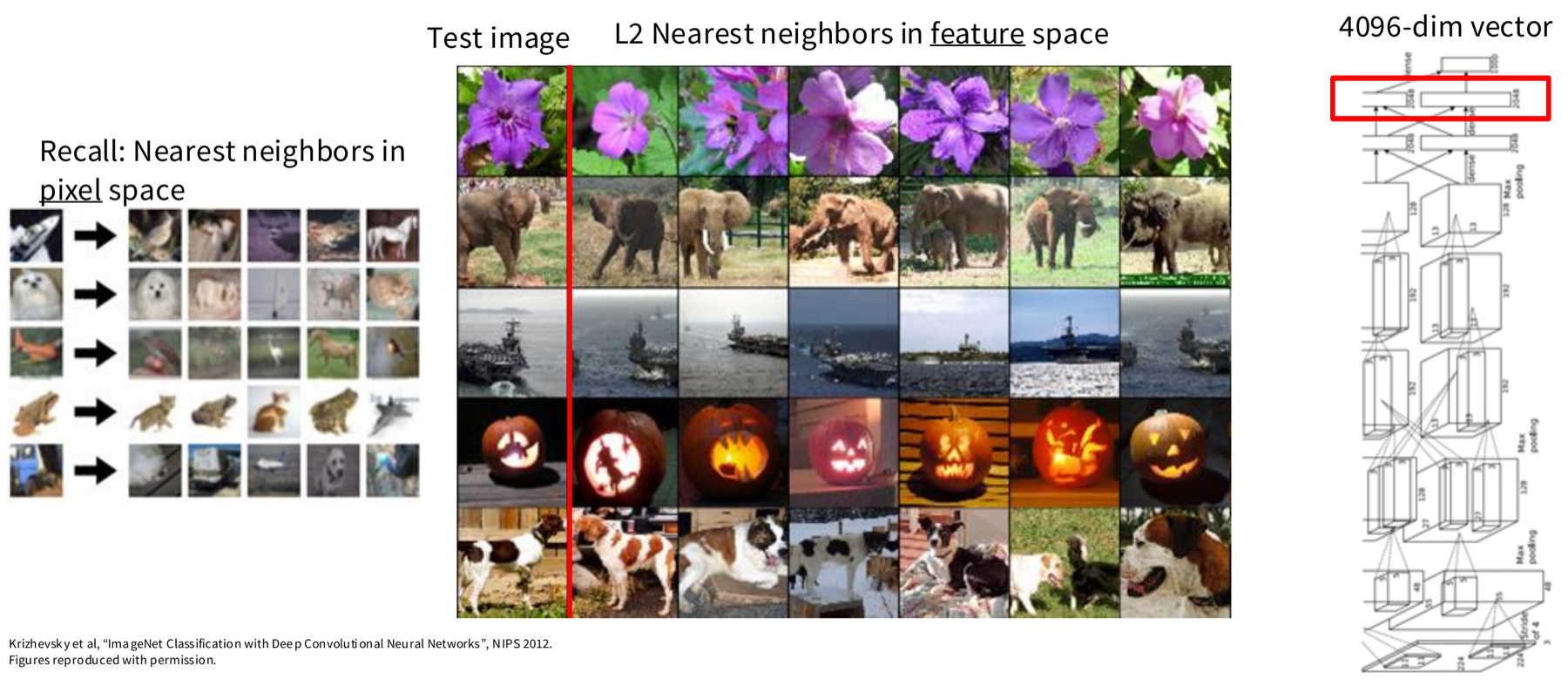
Slide from Stanford CS231n (2026), Lecture 12, p. 9. (p. 8 shows the same figure under the title “Last Week: Visualizing and Understanding”.) Figure: Krizhevsky et al. (2012).
A · Self-Supervised Learning
Learned Representations
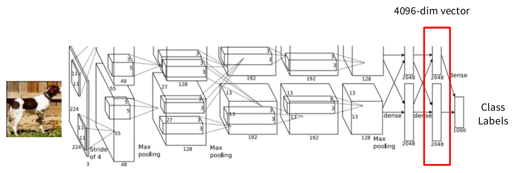
What is the problem with large-scale training?
- We need a lot of labeled data
Is there a way we can train neural networks without the need for huge manually labeled datasets?
Slide from Stanford CS231n (2026), Lecture 12, p. 10. Figure: Krizhevsky et al. (2012); the deck adds “Figures reproduced with permission”.
A · Self-Supervised Learning
Self-Supervised Learning
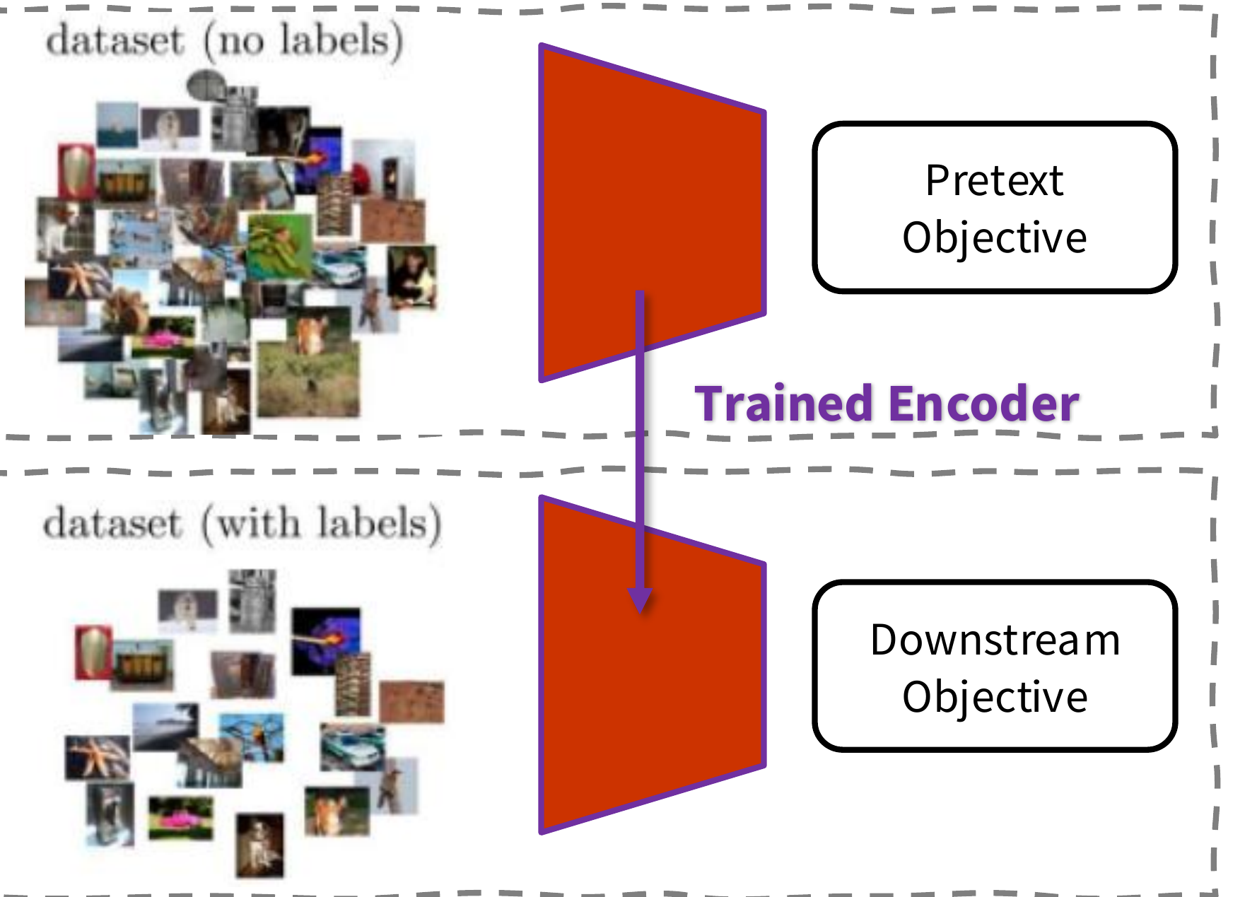
1. Pretext Task
- Define a task based on the data itself
- No manual annotation
- Could be considered an unsupervised task;
- but we learn with supervised learning objectives, e.g., classification or regression.
2. Downstream Task
- The application you care about
- You do not have large datasets
- The dataset is labeled
Slide from Stanford CS231n (2026), Lecture 12, p. 11.
A · Self-Supervised Learning
Self-Supervised Learning – Pretext Task
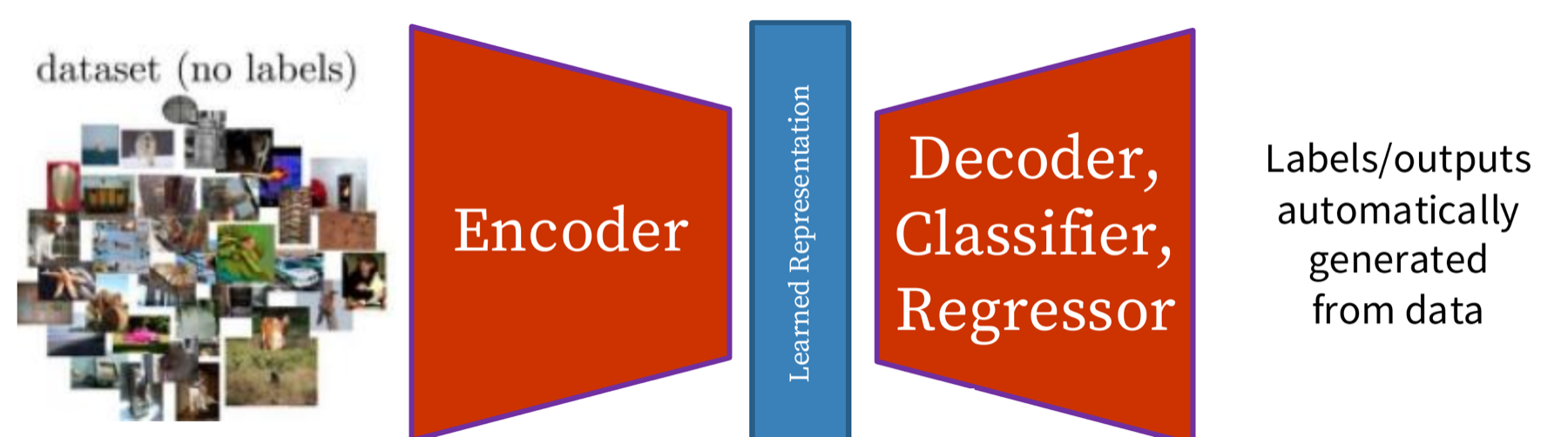
Slide from Stanford CS231n (2026), Lecture 12, p. 12.
A · Self-Supervised Learning
Self-Supervised Learning – Downstream Task (supervised)
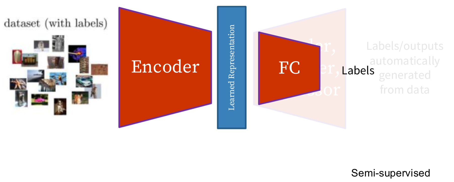
Slide from Stanford CS231n (2026), Lecture 12, p. 13.
A · Self-Supervised Learning
Self-supervised pretext tasks
Example: learn to predict image transformations / complete corrupted images
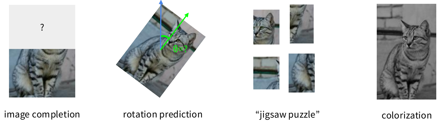
- Solving the pretext tasks allow the model to learn good features.
- We can automatically generate labels for the pretext tasks.
Slide from Stanford CS231n (2026), Lecture 12, p. 14.
A · Self-Supervised Learning
How to evaluate a self-supervised learning method?
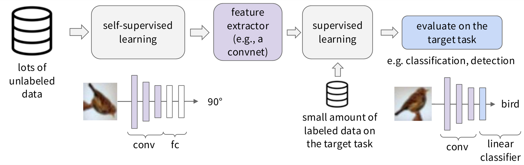
1. Learn good feature extractors from self-supervised pretext tasks, e.g., predicting image rotations
2. Attach a shallow network on the feature extractor; train the shallow network on the target task with small amount of labeled data
Slide from Stanford CS231n (2026), Lecture 12, pp. 16–17. One animation; its final state.
A · Self-Supervised Learning
Broader picture
Today’s lecture
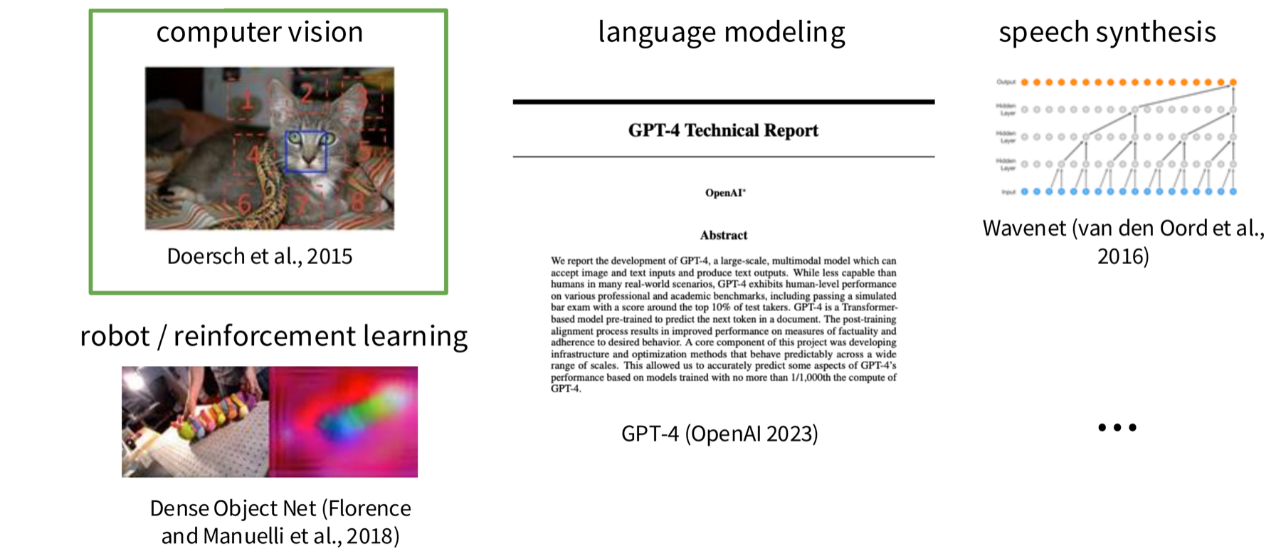
Slide from Stanford CS231n (2026), Lecture 12, p. 18. Works shown: Doersch et al. (2015); OpenAI (2023); van den Oord et al. (2016); Florence et al. (2018).
A · Pretext tasks from image transformations
Pretext task: predict rotations
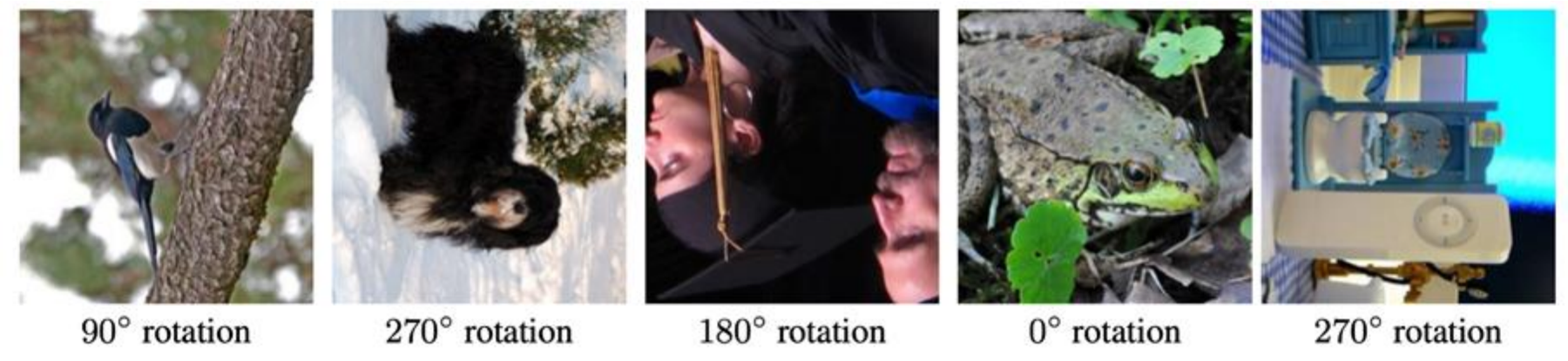
Hypothesis: a model could recognize the correct rotation of an object only if it has the “visual commonsense” of what the object should look like unperturbed.
Slide from Stanford CS231n (2026), Lecture 12, p. 21. Figure: Gidaris et al. (2018).
A · Pretext tasks from image transformations
Pretext task: predict rotations
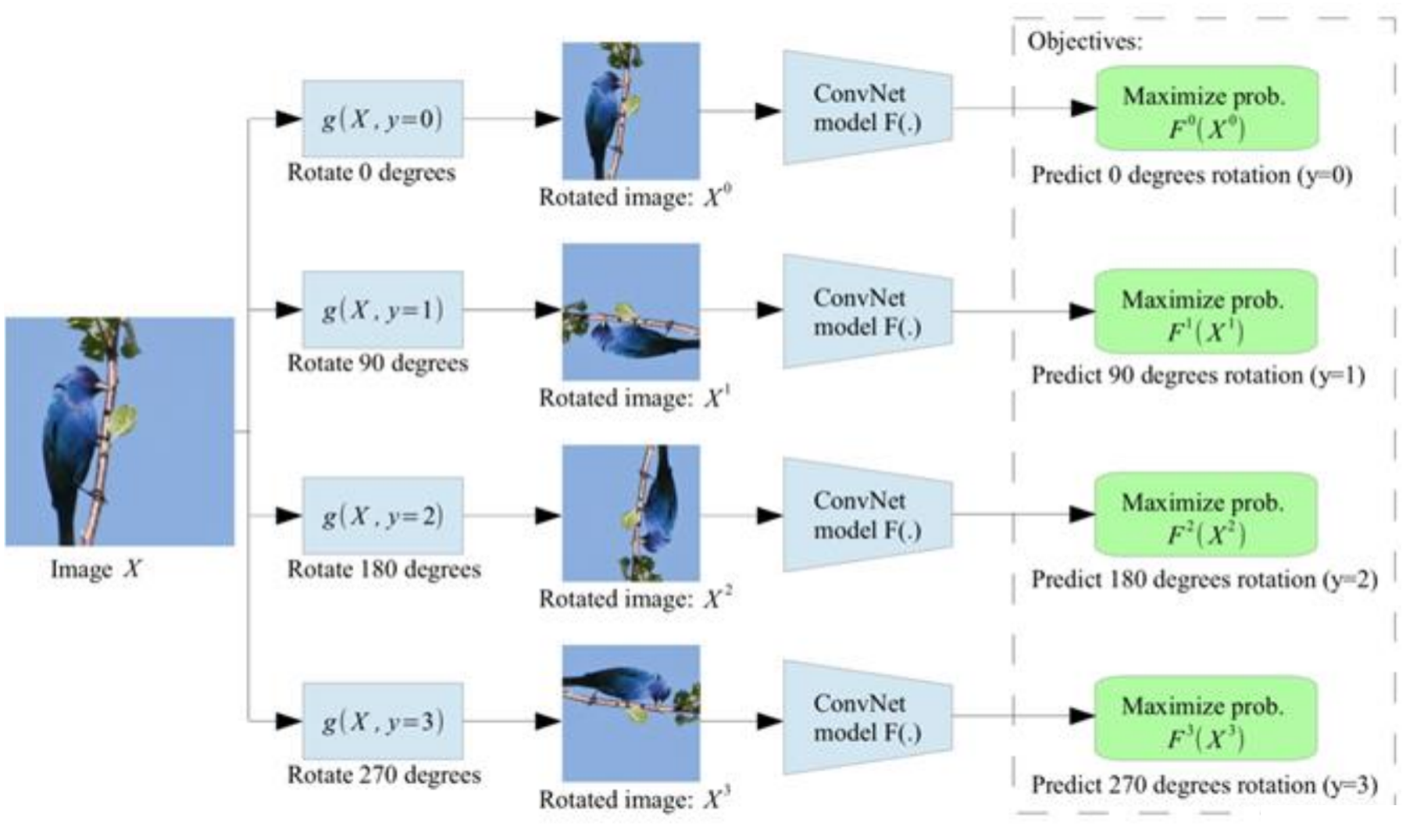
Self-supervised learning by rotating the entire input images.
The model learns to predict which rotation is applied (4-way classification)
Slide from Stanford CS231n (2026), Lecture 12, pp. 22–23. One animation; its final state. Figure: Gidaris et al. (2018).
A · Pretext tasks from image transformations
Evaluation on semi-supervised learning
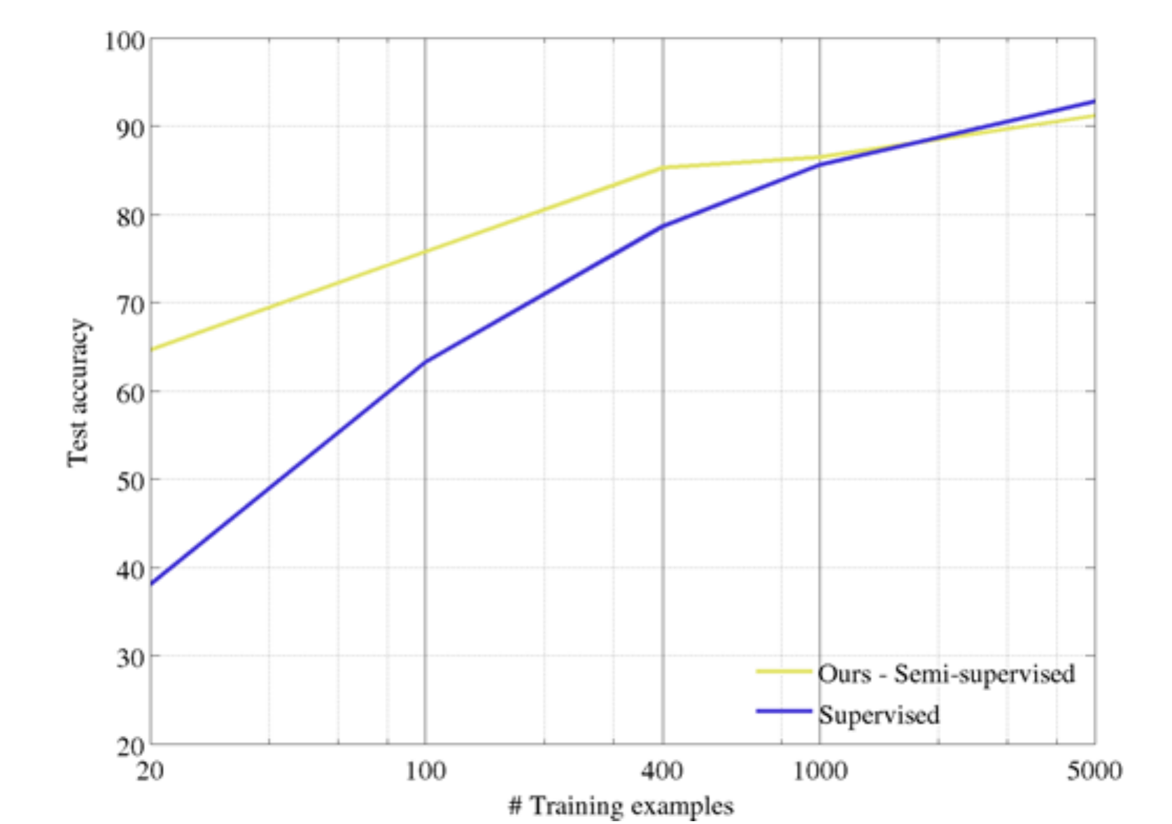
Self-supervised learning on CIFAR10 (entire training set).
Freeze conv1 + conv2
Learn conv3 + linear layers with subset of labeled CIFAR10 data (classification).
Slide from Stanford CS231n (2026), Lecture 12, p. 24. Figure: Gidaris et al. (2018).
A · Pretext tasks from image transformations
Transfer learned features to supervised learning
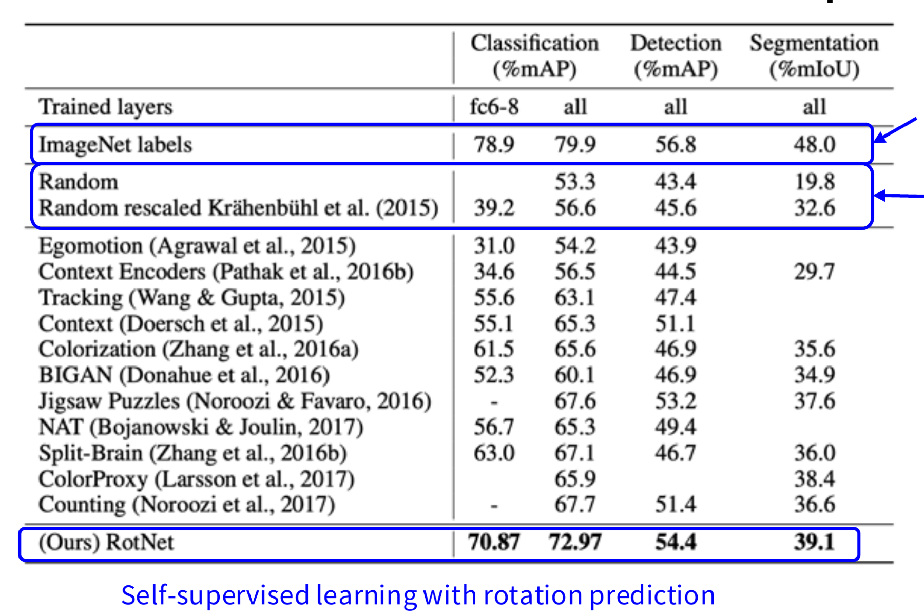
Full supervised learning
No pretraining
Self-supervised learning on ImageNet (entire training set [1,281,167 images]) with AlexNet.
Finetune on labeled data from Pascal VOC 2007 [trainval: 5,011 images].
Slide from Stanford CS231n (2026), Lecture 12, p. 25. Figure: Gidaris et al. (2018). Image counts in brackets (added): ILSVRC 2012 training set, image-net.org; VOC 2007 trainval, Ultralytics VOC dataset page. Retrieved 3 Nov 2026.
A · Pretext tasks from image transformations
Visualize learned visual attentions
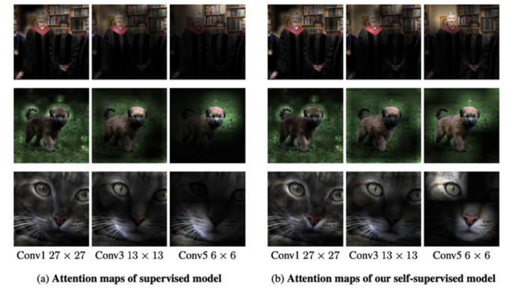
Self-supervised learned attention has better interpretation.
A · Pretext tasks from image transformations
Pretext task: predict relative patch locations
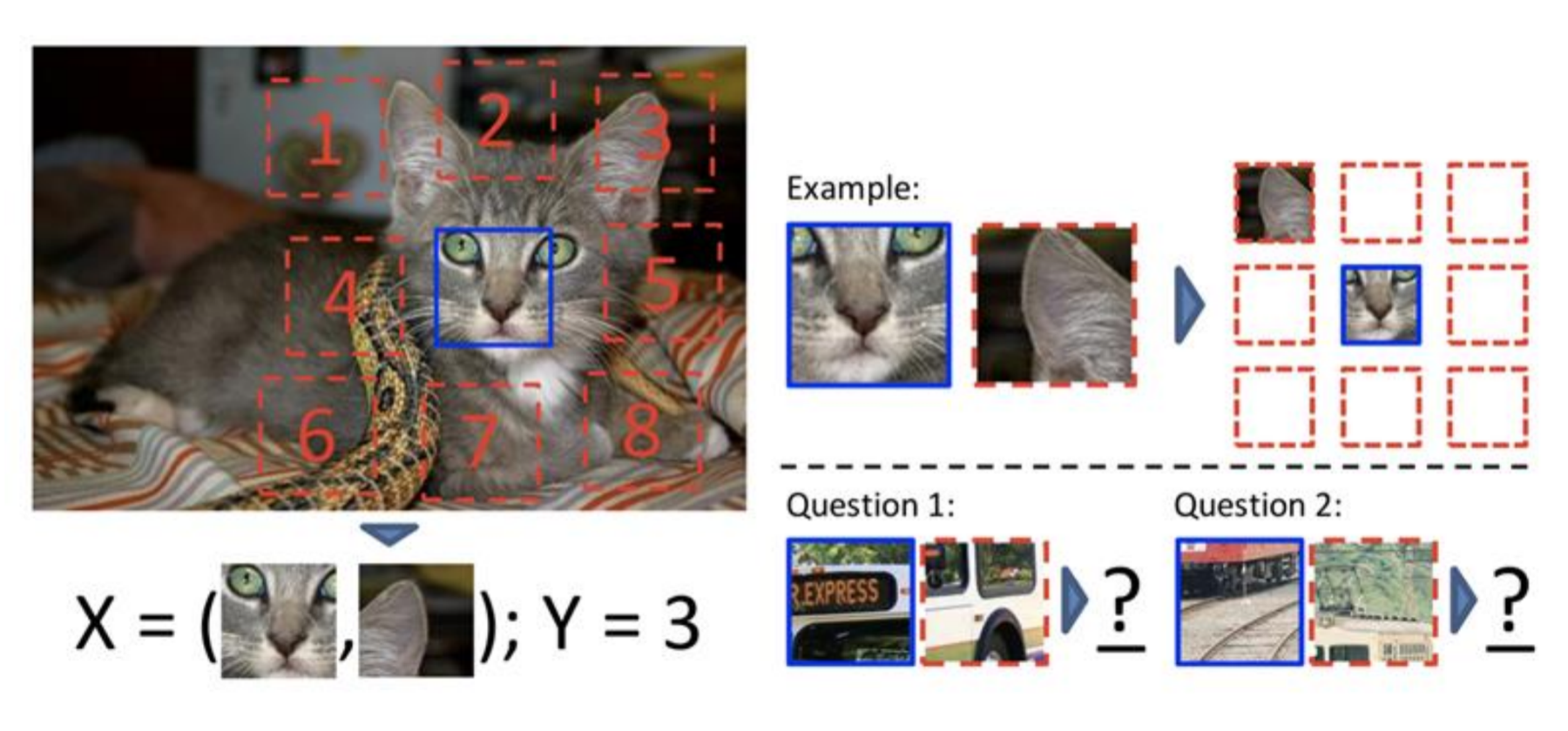
Slide from Stanford CS231n (2026), Lecture 12, p. 27. Figure: Doersch et al. (2015).
A · Pretext tasks from image transformations
Pretext task: solving “jigsaw puzzles”
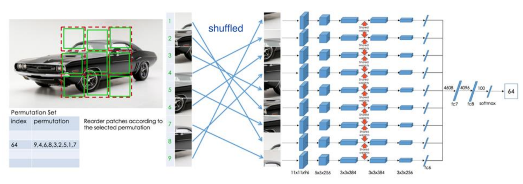
The model predicts the arrangement of the shuffled tiles (the index of the permutation -- learn the relation of patches in the image), not the object category.
Slide from Stanford CS231n (2026), Lecture 12, p. 28. Figure: Noroozi & Favaro (2016), Fig. 3
A · Pretext tasks from image transformations
Pretext task: predict missing pixels (inpainting)
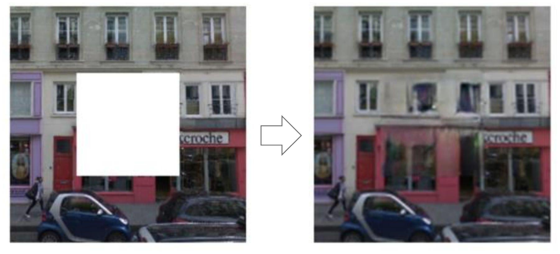
Context Encoders: Feature Learning by Inpainting (Pathak et al., 2016)
Slide from Stanford CS231n (2026), Lecture 12, p. 30. Figure: Pathak et al. (2016).
A · Pretext tasks from image transformations
Learning to inpaint by reconstruction
Auto Encoder
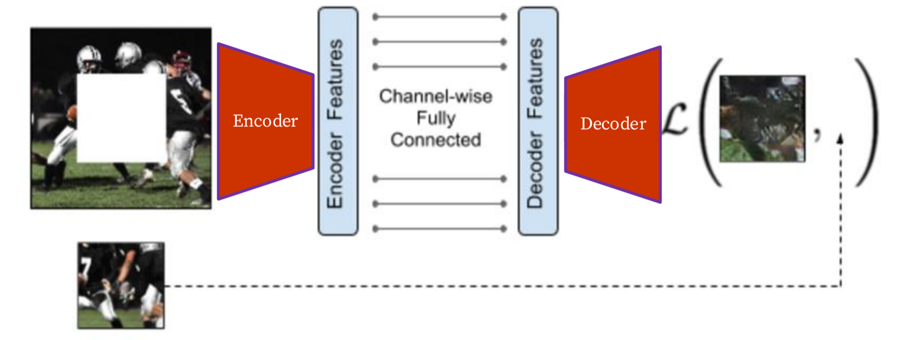
Learning to reconstruct the missing pixels
Slide from Stanford CS231n (2026), Lecture 12, p. 31. Figure: Pathak et al. (2016).
A · Pretext tasks from image transformations
Inpainting evaluation
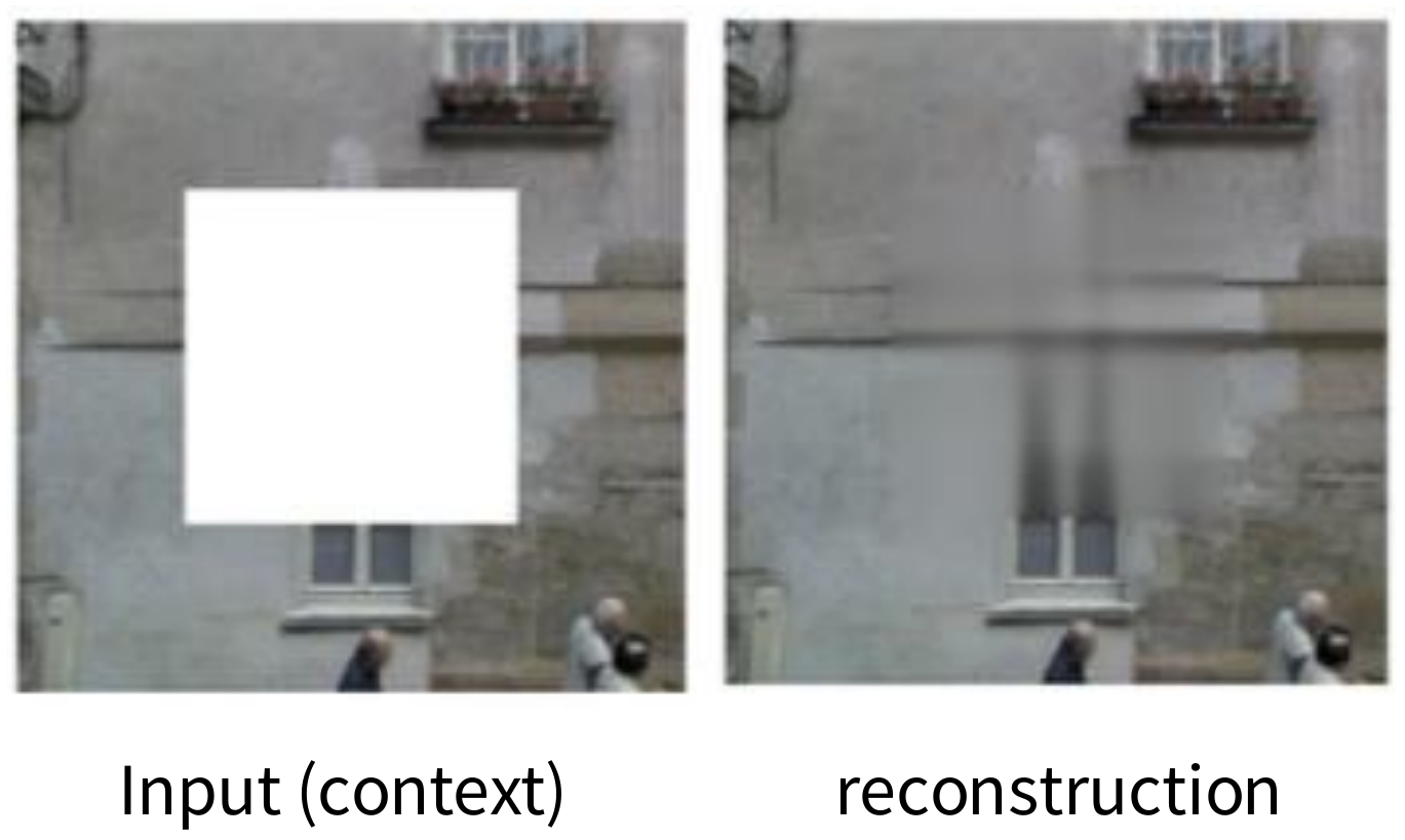
Slide from Stanford CS231n (2026), Lecture 12, p. 32. Figure: Pathak et al. (2016).
A · Pretext tasks from image transformations
Inpainting evaluation
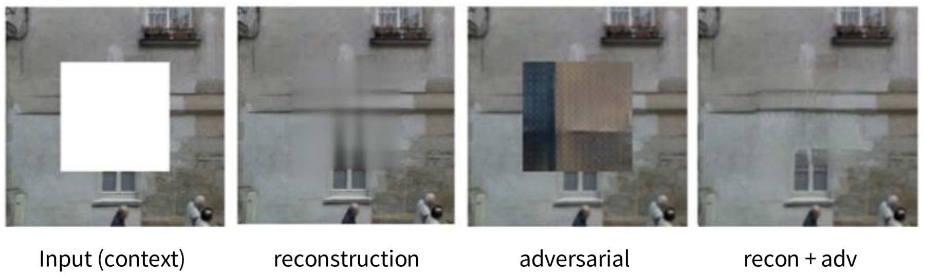
Slide from Stanford CS231n (2026), Lecture 12, p. 34. Figure: Pathak et al. (2016).
A · Pretext tasks from image transformations
Transfer learned features to supervised learning
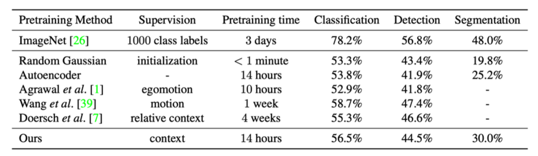
Self-supervised learning on ImageNet training set, transfer to classification (Pascal VOC 2007), detection (Pascal VOC 2007), and semantic segmentation (Pascal VOC 2012)
Slide from Stanford CS231n (2026), Lecture 12, p. 35. Table: Pathak et al. (2016).
A · Pretext tasks from image transformations
Pretext task: image coloring
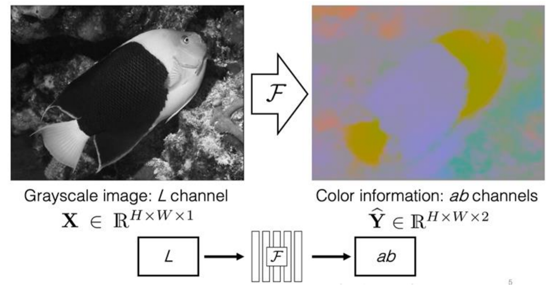
Slide from Stanford CS231n (2026), Lecture 12, p. 36. The deck credits “Richard Zhang / Phillip Isola”. See Zhang et al. (2016).
A · Pretext tasks from image transformations
Pretext task: image coloring
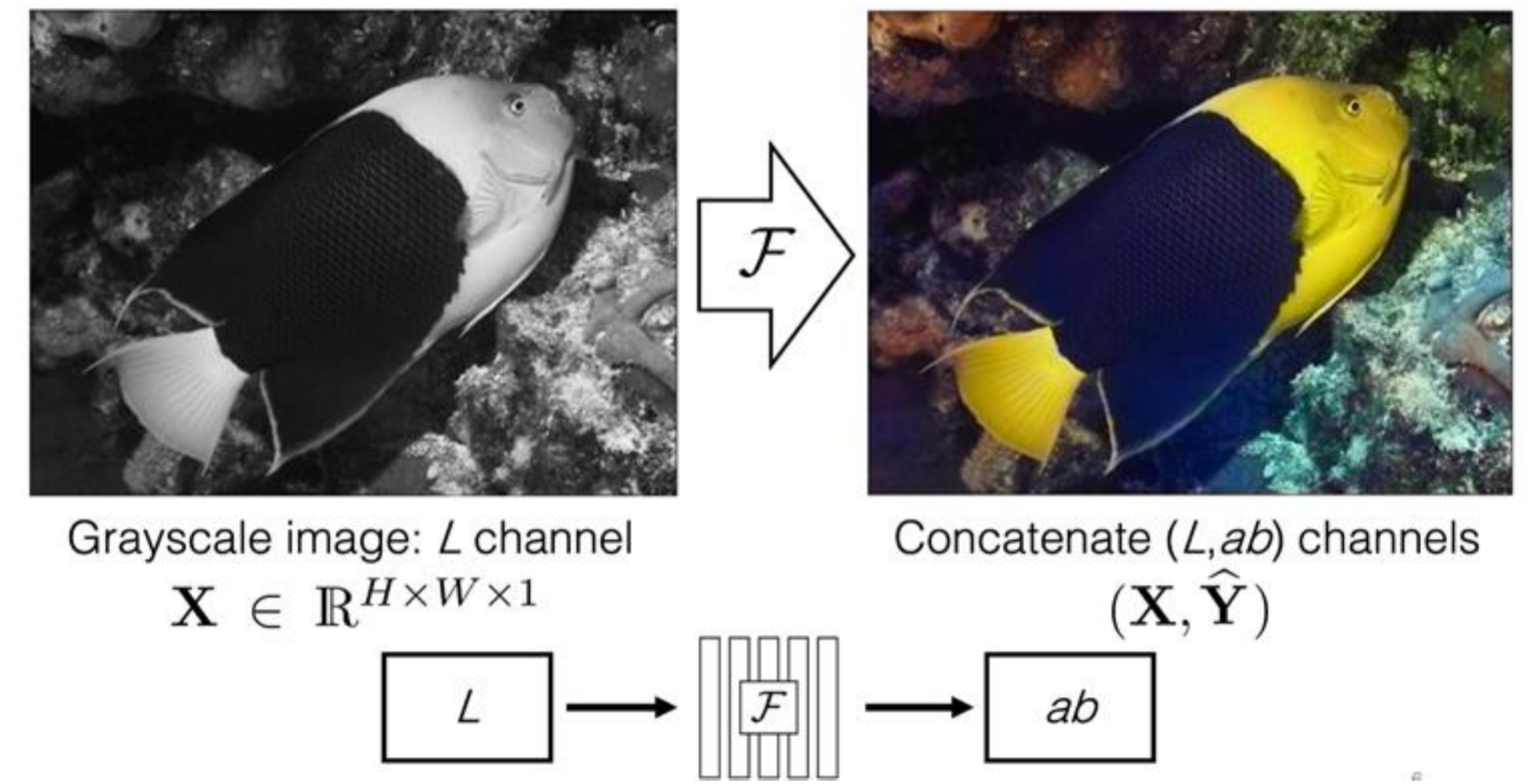
Slide from Stanford CS231n (2026), Lecture 12, p. 37. The deck credits “Richard Zhang / Phillip Isola”. See Zhang et al. (2016).
A · Pretext tasks from image transformations
Learning features from colorization: Split-brain Autoencoder
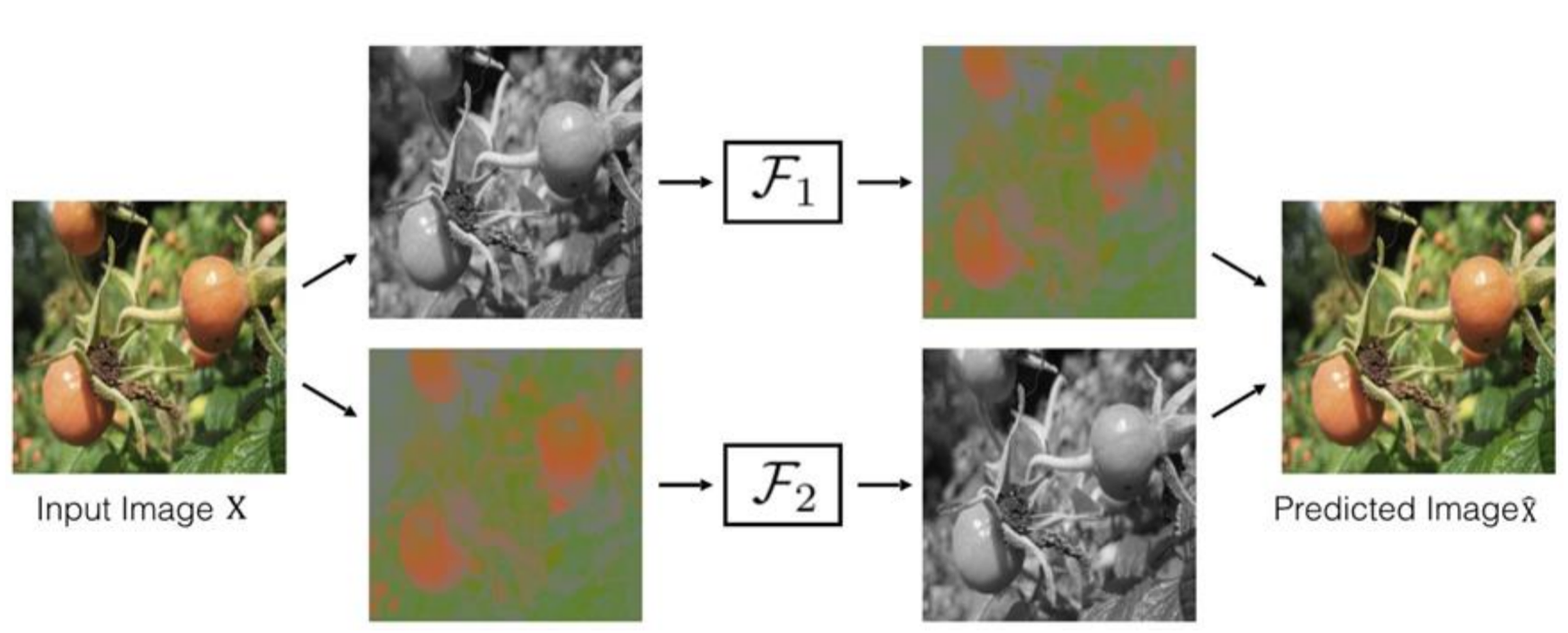
F1 sees only the grayscale channel and predicts the colour channels. F2 sees only the colour channels and predicts the grayscale channel. Each network predicts what the other one sees.
Slide from Stanford CS231n (2026), Lecture 12, p. 38. The deck credits “Richard Zhang / Phillip Isola”. Figure: Zhang et al. (2017). The caption under the figure is added.
A · Pretext tasks from image transformations
Learning features from colorization: Split-brain Autoencoder
Idea: cross-channel predictions
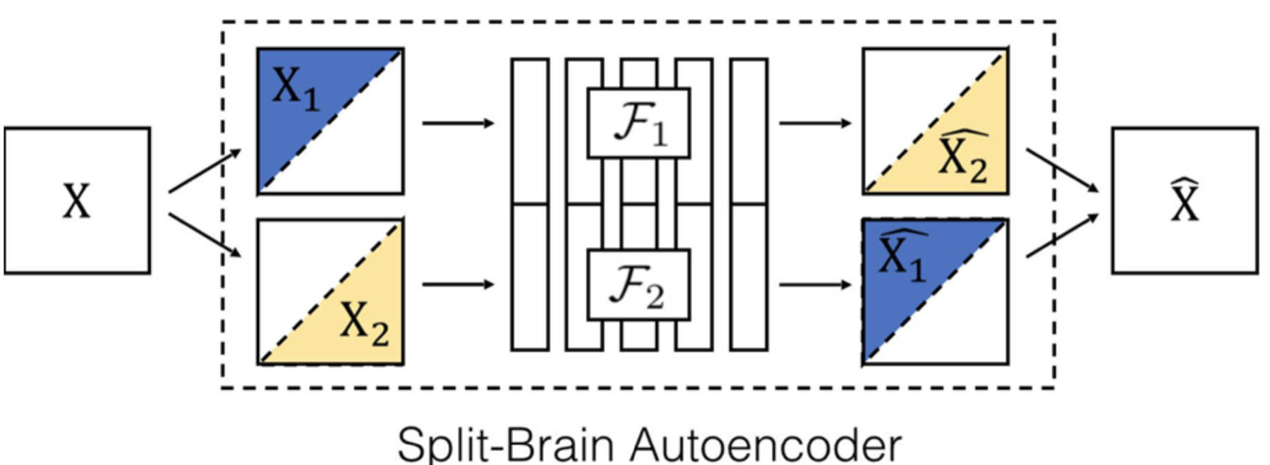
Slide from Stanford CS231n (2026), Lecture 12, p. 39. The deck credits “Richard Zhang / Phillip Isola”. Figure: Zhang et al. (2017).
A · Pretext tasks from image transformations
Transfer learned features to supervised learning
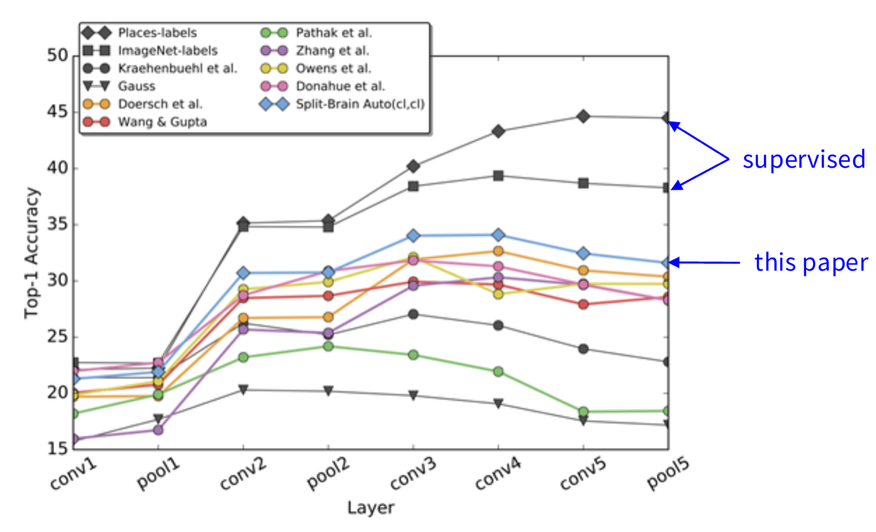
Self-supervised learning on ImageNet (entire training set).
Use concatenated features from F₁ and F₂
Labeled data is from the Places (Zhou 2016).
Slide from Stanford CS231n (2026), Lecture 12, p. 40. Figure: Zhang et al. (2017). Places: Zhou et al. (2016).
A · Pretext tasks from image transformations
Pretext task: image coloring
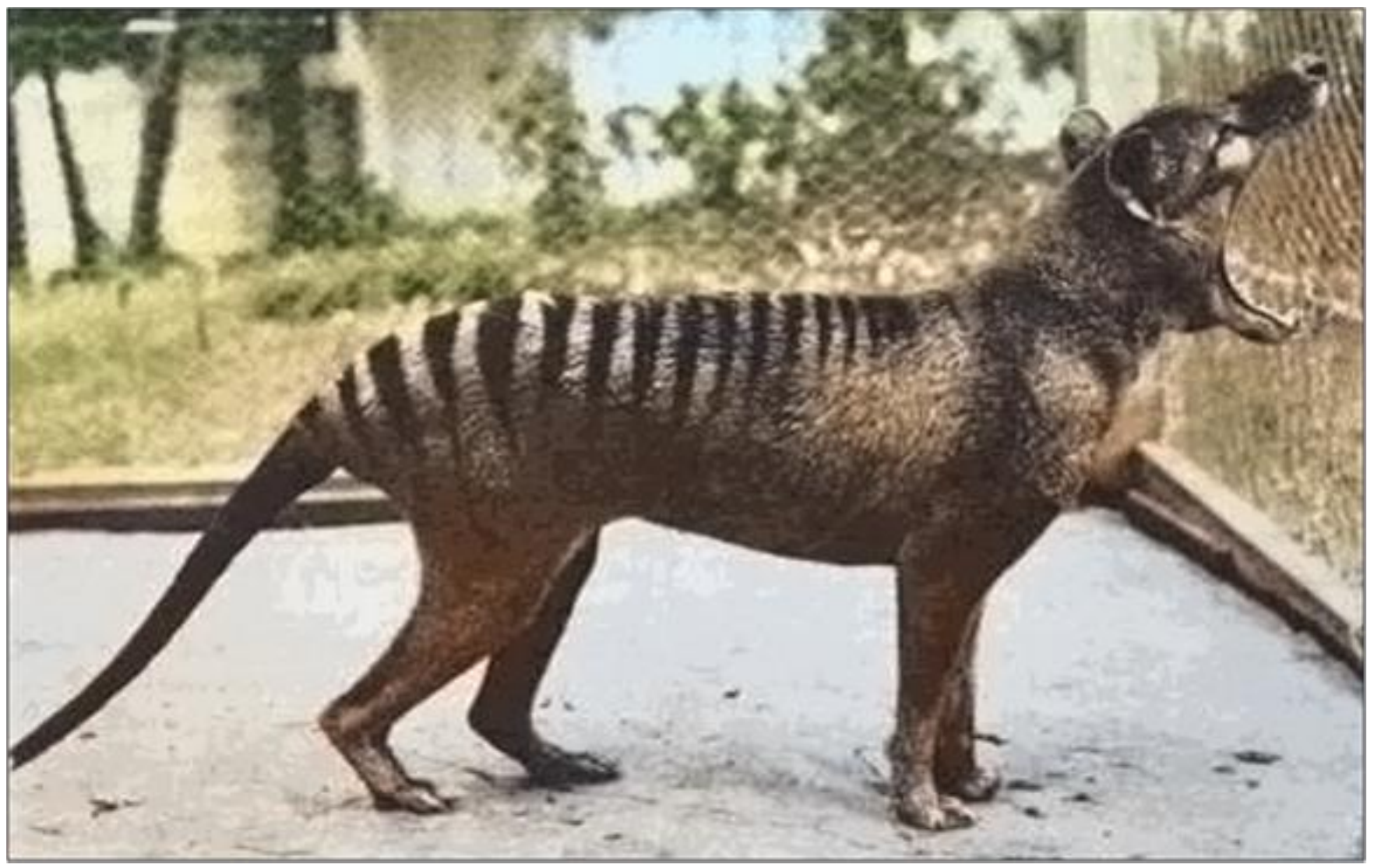
Slide from Stanford CS231n (2026), Lecture 12, p. 41. The deck credits “Richard Zhang / Phillip Isola”. See Zhang et al. (2016).
A · Pretext tasks from image transformations
Pretext task: image coloring
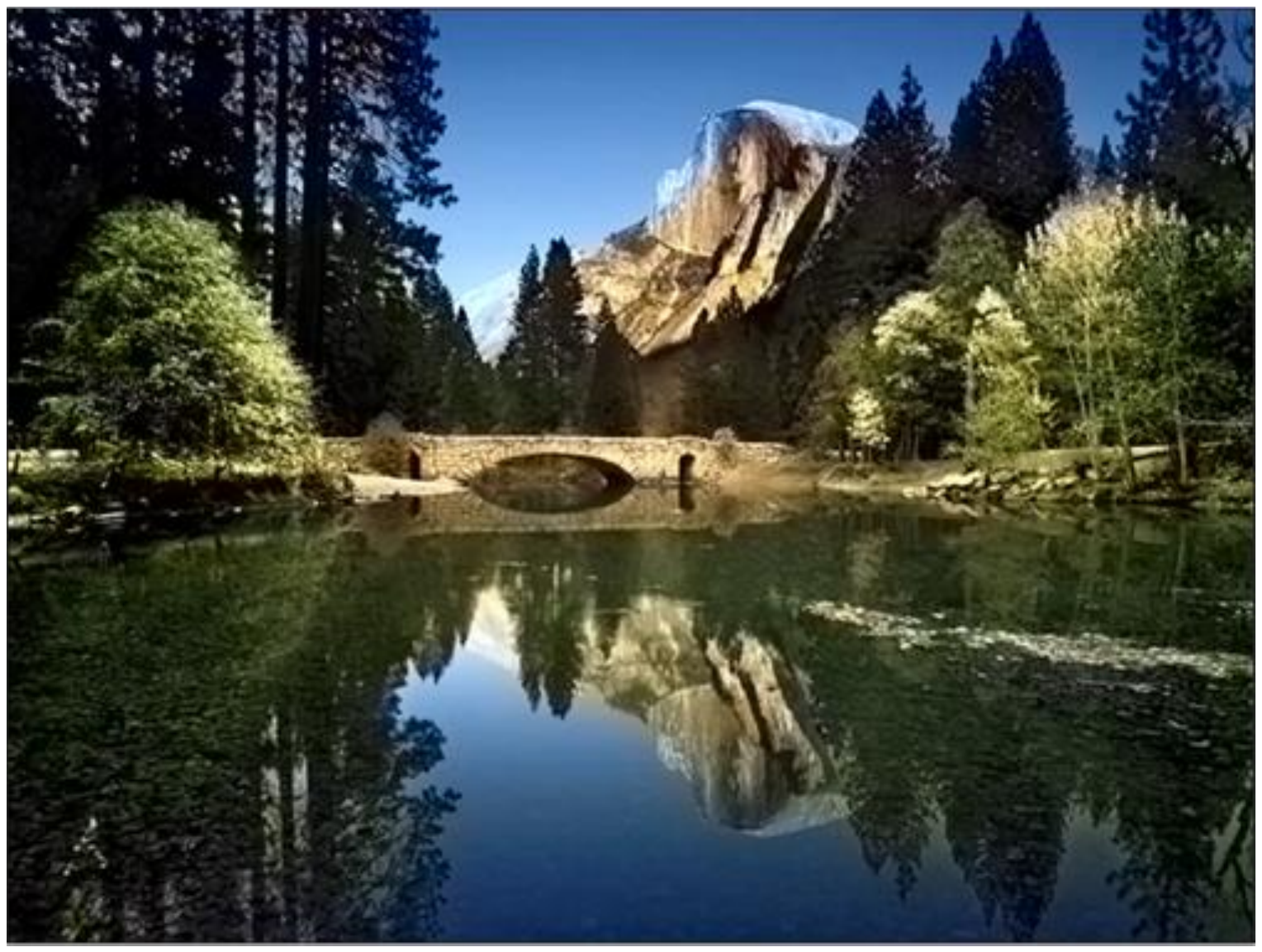
Slide from Stanford CS231n (2026), Lecture 12, p. 42. The deck credits “Richard Zhang / Phillip Isola”. See Zhang et al. (2016).
A · Pretext tasks from image transformations
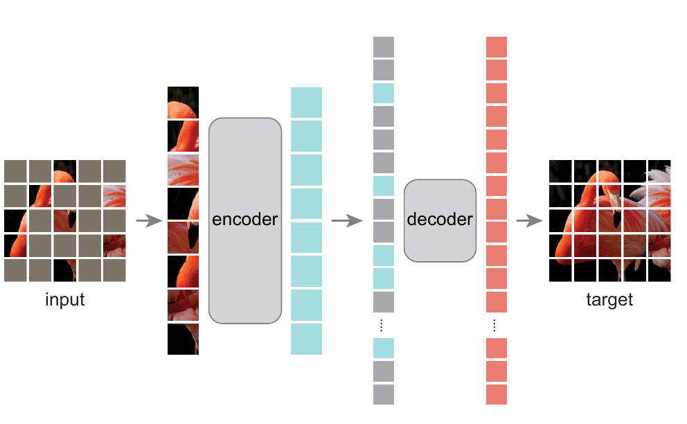
Masked Auto Encoders (MAE)
Scaling inpainting idea: Reconstruction with a larger masked portion
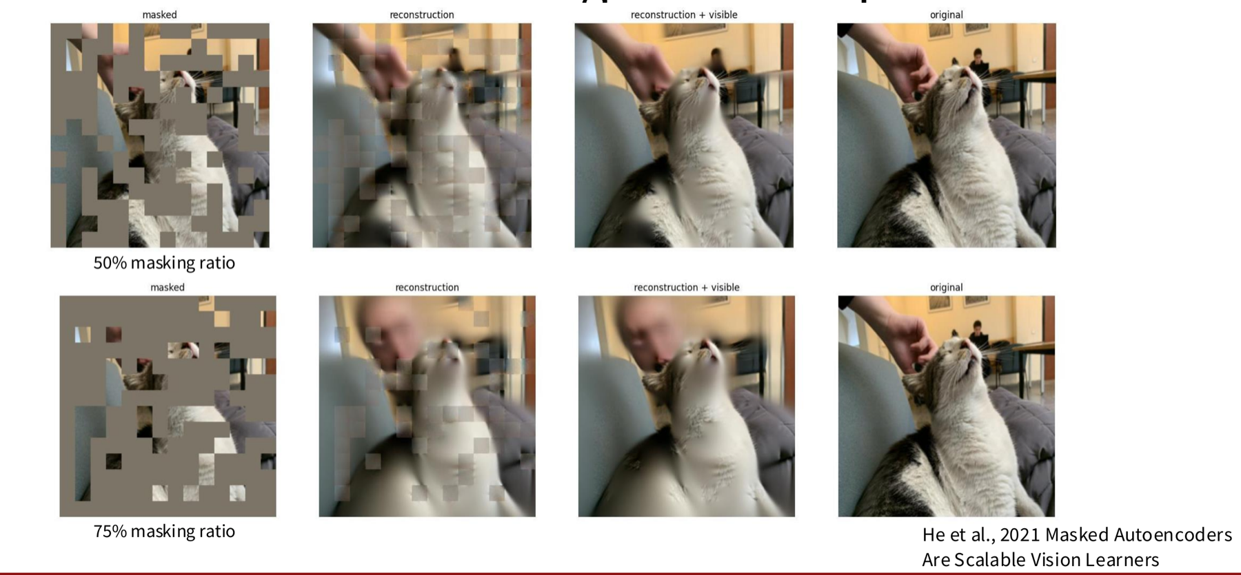
Slide from Stanford CS231n (2026), Lecture 12, p. 48. Figure: He et al. (2022)
A · Pretext tasks from image transformations
Masked Auto Encoders (MAE)
Slide from Stanford CS231n (2026), Lecture 12, p. 49. Figure: He et al. (2022), Fig. 1.
A · Pretext tasks from image transformations
Masking Methods
- Similar to the original ViT,
divide the input into non-overlapping patches. - Uniformly sample a very large proportion (75%) of these patches and mask them
- Masking a high ratio makes predicting the task challenging and meaningful.
- Also, not using mask tokens and picking a high sampling ratio (masking most of the image, e.g., 75%, and sampling a small visible portion, e.g., 25%, to feed into the encoder) enables the encoder to be very large.
from the paper
Slide from Stanford CS231n (2026), Lecture 12, p. 50. Figure: He et al. (2022), Fig. 1 (the page labels it “Figure 6”).
A · Pretext tasks from image transformations
MAE Encoder
- The encoder only operates
on unmasked patches (25%) - Embeds the patches by linear projection
and add positional embeddings - Uses transformer blocks
from the paper
- Since the input patches are a small part of the input, the encoder is chosen to be very large. (encoder has over 9 times computations per token vs decoder)
Slide from Stanford CS231n (2026), Lecture 12, p. 51. Figure: He et al. (2022), Fig. 1 (the page labels it “Figure 6”).
A · Pretext tasks from image transformations
MAE Decoder
- Merges the encoder outputs with the shared mask tokens in previously masked places, adding positional encodings to them.
- Uses transformer blocks, followed by a linear projection for finalizing pixel reconstruction.
from the paper
- Is solely responsible for reconstruction, meaning it is not used post-training. Hence, it is independent of the encoder design, making it flexible (unlike traditional AEs or UNet). This is an asymmetrical autoencoder design.
Slide from Stanford CS231n (2026), Lecture 12, p. 52. Figure: He et al. (2022), Fig. 1 (the page labels it “Figure 6”).
A · Pretext tasks from image transformations
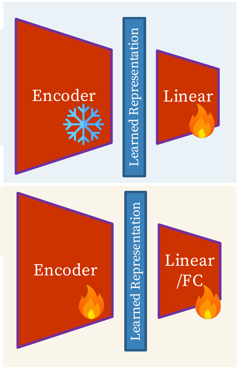
Linear Probing vs Full Fine-tuning
- In linear probing, the pre-trained model is fixed, and only one linear layer is added at the end, to predict the labels (or produce the output). This method is used to assess the quality of representations from a pre-trained feature extraction model.
- In fine-tuning, pre-trained model is further trained (not fixed), and one or more layers, possibly with non-linearities are added.
- linear probing: provides a measure of representation quality of a pre-training in restricted conditions
- fine-tuning: exploits models near-true potential to adopt for new tasks
Slide from Stanford CS231n (2026), Lecture 12, p. 54; diagrams cropped from the same page.
A · Pretext tasks from image transformations
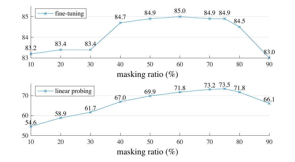
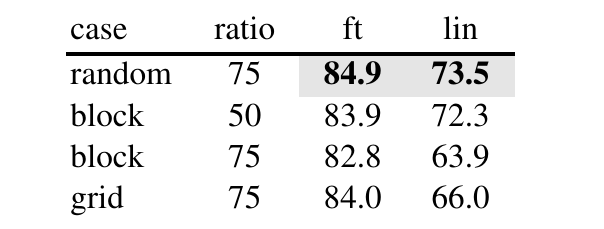
Ablation Studies
So many modeling/
- Masking ratio
- Decoder depth
- Decoder width
- Mask token (used or not in encoder)
- Reconstruction target
- Data augmentation
- Mask sampling method
- Training schedule
Slide from Stanford CS231n (2026), Lecture 12, p. 55 (first of two slides). Figure: He et al. (2022), Fig. 5 (ViT-L).
A · Pretext tasks from image transformations
Ablation Studies
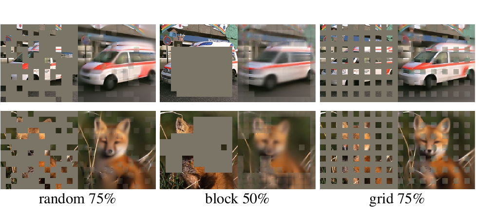
Slide from Stanford CS231n (2026), Lecture 12, p. 55 (second of two slides). Figures: He et al. (2022), Table 1f and Fig. 6 (ViT-L; ft: fine-tuning, lin: linear probing).
A · Pretext tasks from image transformations
Masked Autoencoder – Comparisons
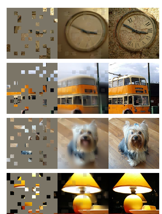
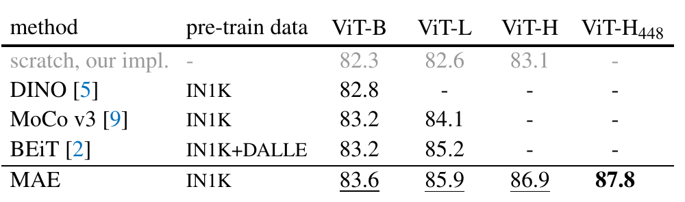
Slide from Stanford CS231n (2026), Lecture 12, p. 56. Figures: He et al. (2022), Fig. 2 (first column; 80% masked) and Table 3.
A · Contrastive representation learning
Pretext tasks from image transformations
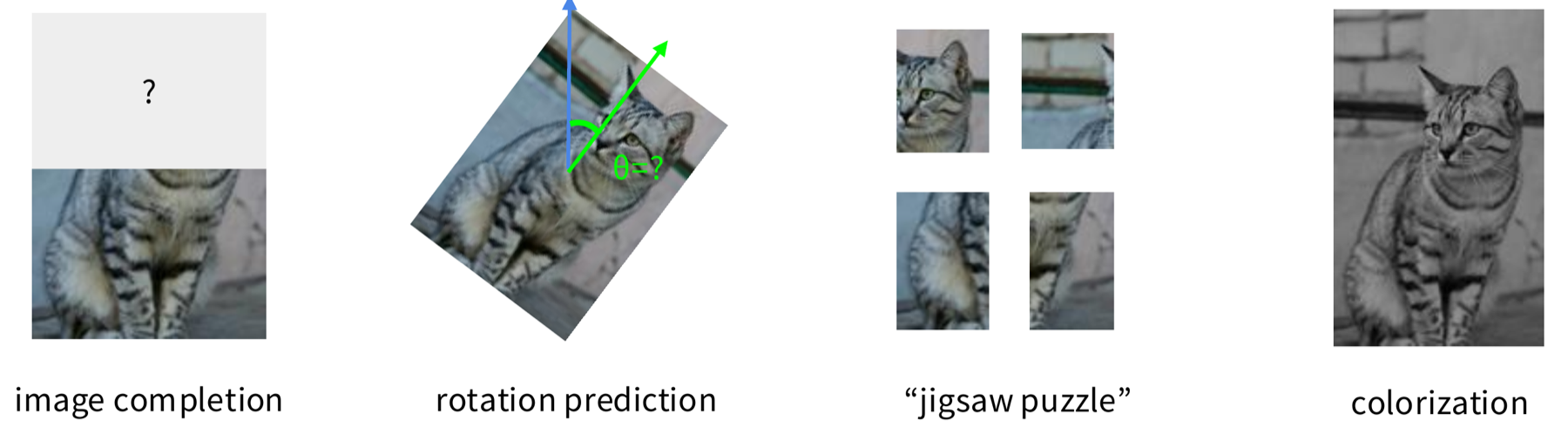
Learned representations may be tied to a specific pretext task!
Can we come up with a more general pretext task?
Slide from Stanford CS231n (2026), Lecture 12, p. 59.
A · Contrastive representation learning
A more general pretext task?
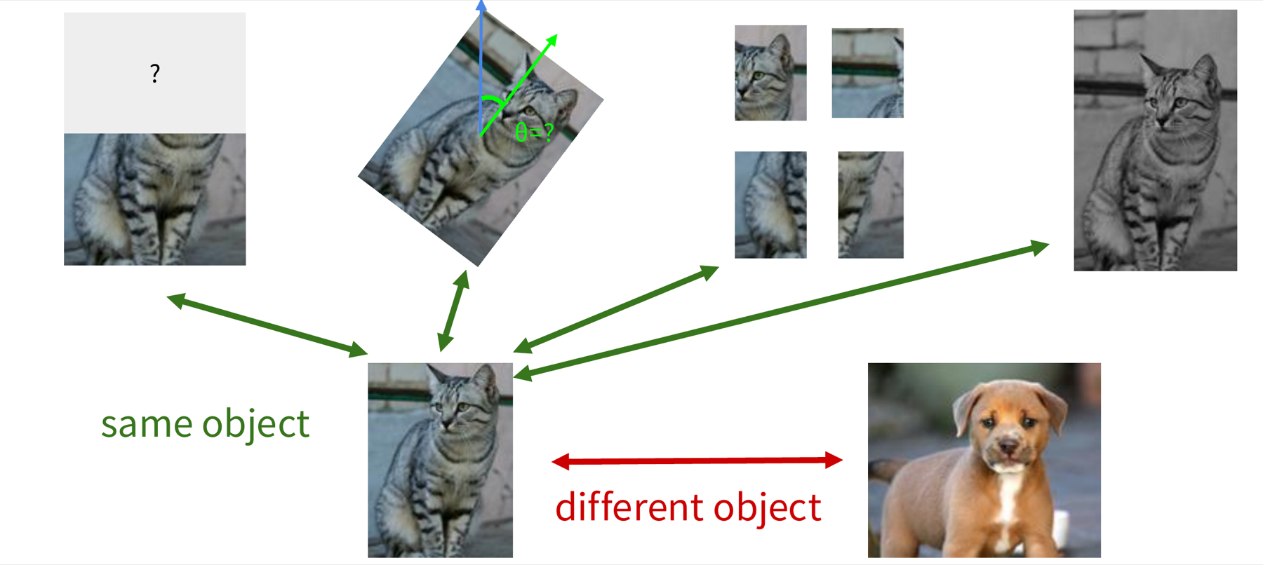
Slide from Stanford CS231n (2026), Lecture 12, pp. 60–61. One animation; its final state.
A · Contrastive representation learning
Contrastive Representation Learning
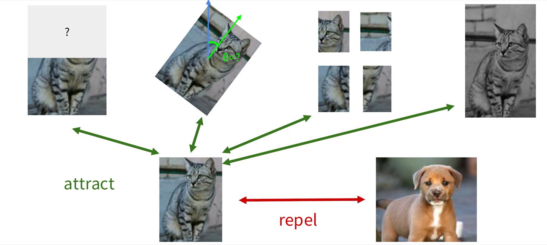
Slide from Stanford CS231n (2026), Lecture 12, pp. 62, 64. Page 64 repeats page 62 after the deck’s agenda page.
B · Intuition and formulation
Contrastive Representation Learning
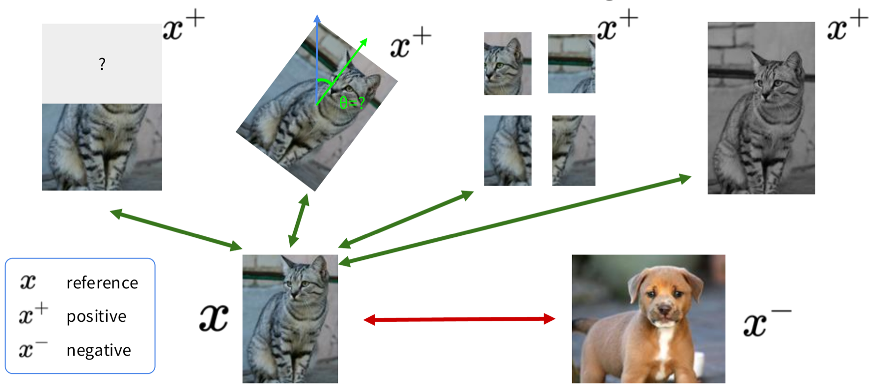
Slide from Stanford CS231n (2026), Lecture 12, p. 65.
B · Intuition and formulation
A formulation of contrastive learning
Loss function given 1 positive sample and N - 1 negative samples:
This seems familiar …
Cross entropy loss for a N-way softmax classifier!
I.e., learn to find the positive sample from the N samples
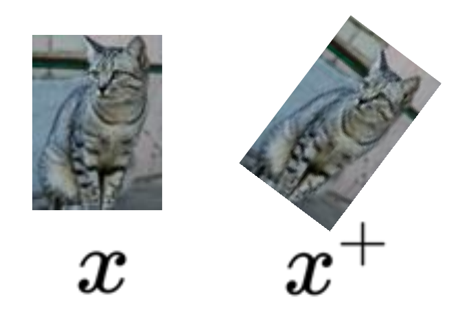
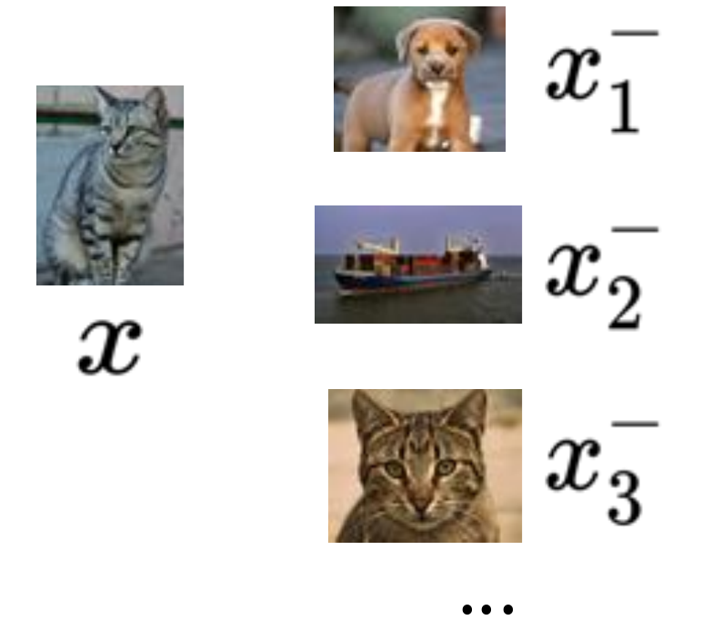
Slide from Stanford CS231n (2026), Lecture 12, pp. 67–70 (one build, final state). Photos cropped from p. 68.
B · Instance contrastive learning: SimCLR and MOCO
SimCLR: A Simple Framework for Contrastive Learning
Cosine similarity as the score function:
Use a projection network g(·) to project features to a space where contrastive learning is applied
Generate positive samples through data augmentation:
- random cropping, random color distortion, and random blur.
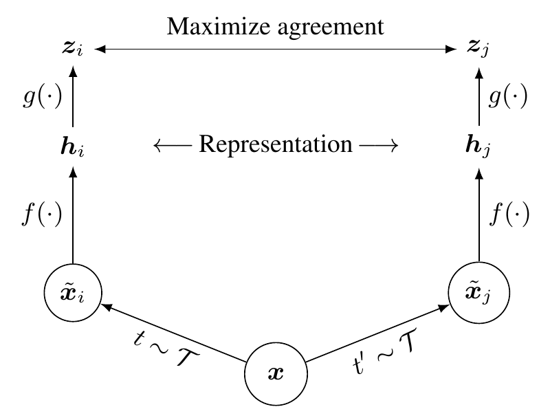
Slide from Stanford CS231n (2026), Lecture 12, p. 72. Source: Chen et al., 2020. Figure: Chen et al. (2020), Fig. 2.
B · Instance contrastive learning: SimCLR and MOCO
SimCLR: generating positive samples from data augmentation
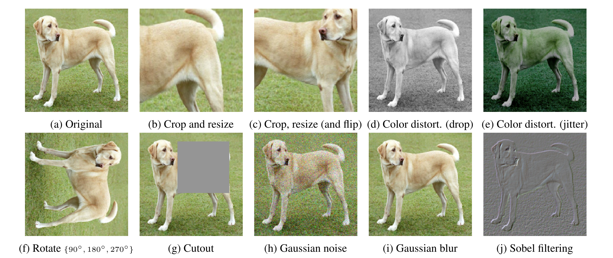
Slide from Stanford CS231n (2026), Lecture 12, p. 73. Source: Chen et al., 2020. Figure: Chen et al. (2020), Fig. 4 (photo: CC BY, Von.grzanka).
B · Instance contrastive learning: SimCLR and MOCO
SimCLR
Generate a positive pair by sampling data augmentation functions
Iterate through and use each of the 2N sample as reference, compute average loss
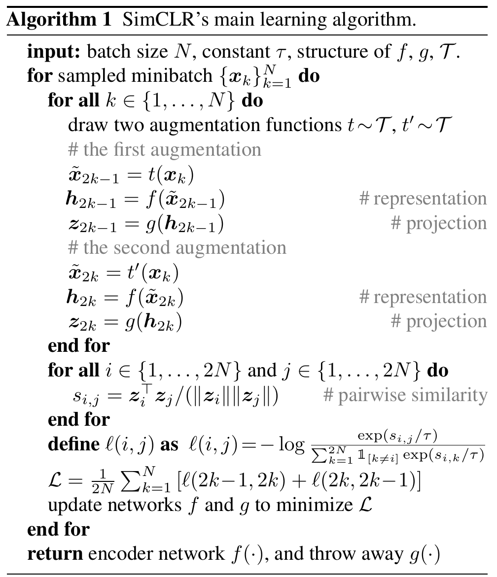
InfoNCE loss:
Use all non-positive samples in the batch as x-
Slide from Stanford CS231n (2026), Lecture 12, pp. 74–76 (one build, final state). Source: Chen et al., 2020. Figure: Algorithm 1.
B · Instance contrastive learning: SimCLR and MOCO
Training linear classifier on SimCLR features
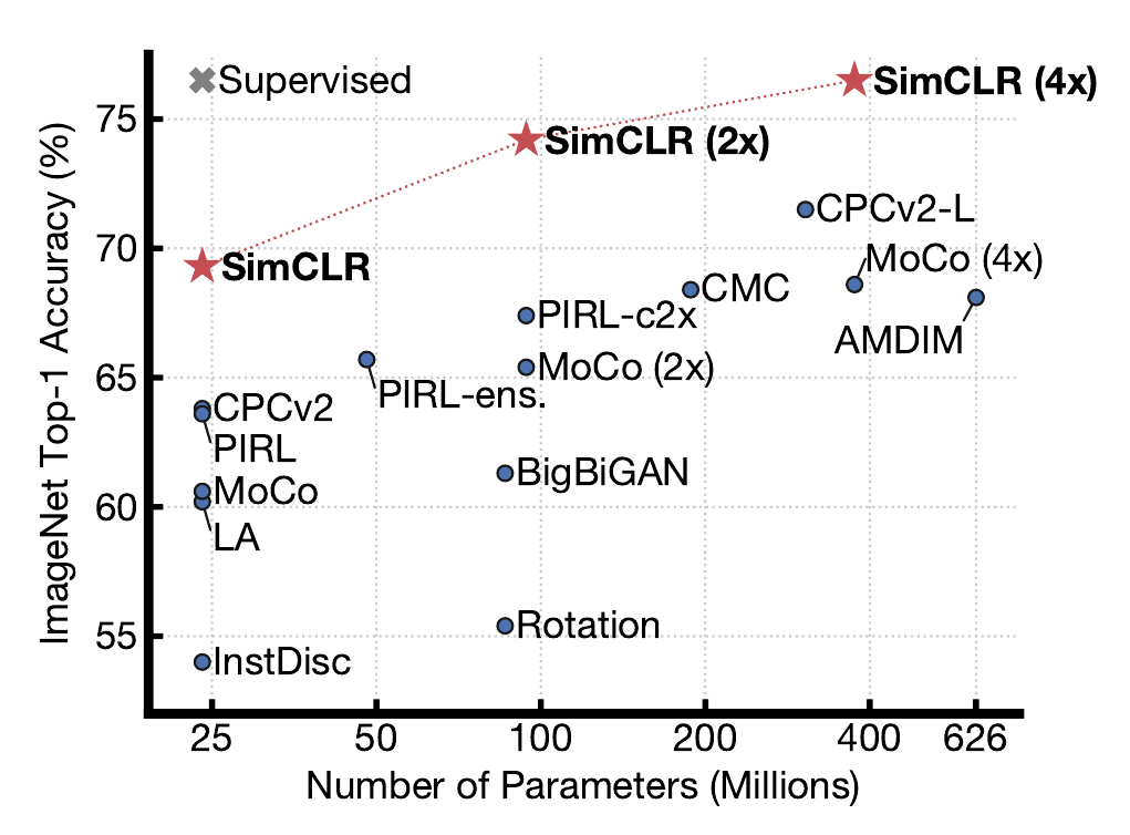
Train feature encoder on ImageNet (entire training set) using SimCLR.
Freeze feature encoder, train a linear classifier on top with labeled data.
Slide from Stanford CS231n (2026), Lecture 12, p. 77. Source: Chen et al., 2020. Figure: Chen et al. (2020), Fig. 1.
B · Instance contrastive learning: SimCLR and MOCO
Semi-supervised learning on SimCLR features
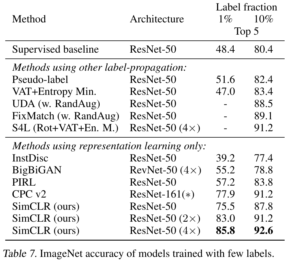
Train feature encoder on ImageNet (entire training set) using SimCLR.
Finetune the encoder with 1% / 10% of labeled data on ImageNet.
Slide from Stanford CS231n (2026), Lecture 12, p. 78. Source: Chen et al., 2020. Table: Chen et al. (2020), Table 7.
B · Instance contrastive learning: SimCLR and MOCO
SimCLR design choices: projection head
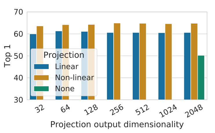
Linear / non-linear projection heads improve representation learning.
A possible explanation:
- contrastive learning objective may discard useful information for downstream tasks
- representation space z is trained to be invariant to data transformation.
- by leveraging the projection head g(·), more information can be preserved in the h representation space
Slide from Stanford CS231n (2026), Lecture 12, p. 79. Source: Chen et al., 2020. Figures: Chen et al. (2020), Figs. 8 and 2.
B · Instance contrastive learning: SimCLR and MOCO
SimCLR design choices: large batch size
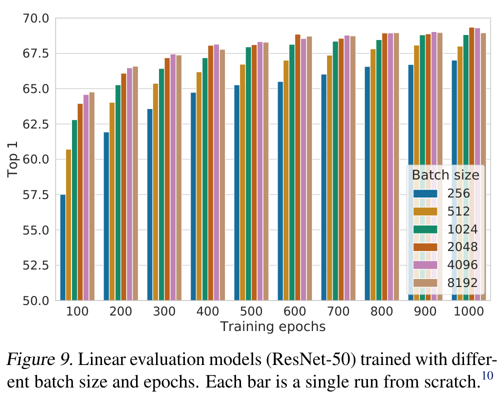
Large training batch size is crucial for SimCLR!
Large batch size causes large memory footprint during backpropagation: requires distributed training on TPUs (ImageNet experiments)
Slide from Stanford CS231n (2026), Lecture 12, p. 80. Source: Chen et al., 2020. Figure: Chen et al. (2020), Fig. 9.
B · Instance contrastive learning: SimCLR and MOCO
Momentum Contrastive Learning (MoCo)
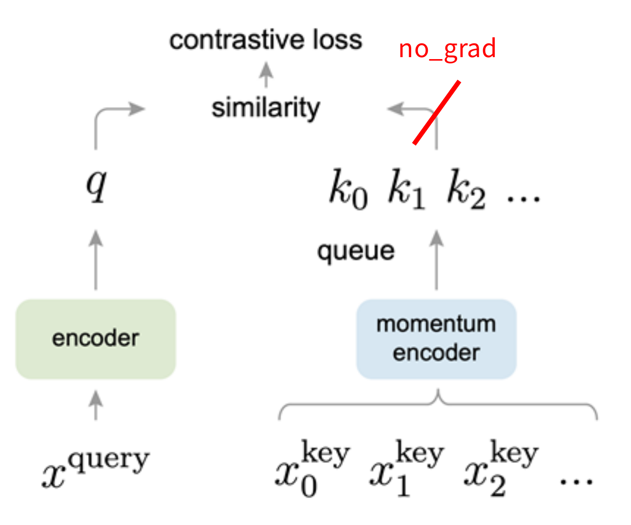
Key differences to SimCLR:
- Keep a running queue of keys (negative samples).
- Compute gradients and update the encoder only through the queries.
- Decouple min-batch size with the number of keys: can support a large number of negative samples.
- The key encoder is slowly progressing through the momentum update rules: \[\theta_k \leftarrow m\theta_k + (1 - m)\theta_q\]
Slide from Stanford CS231n (2026), Lecture 12, pp. 81–82. One animation; its final state. Math retyped. Figure: He et al. (2020), Fig. 1.
B · Instance contrastive learning: SimCLR and MOCO
“MoCo V2”
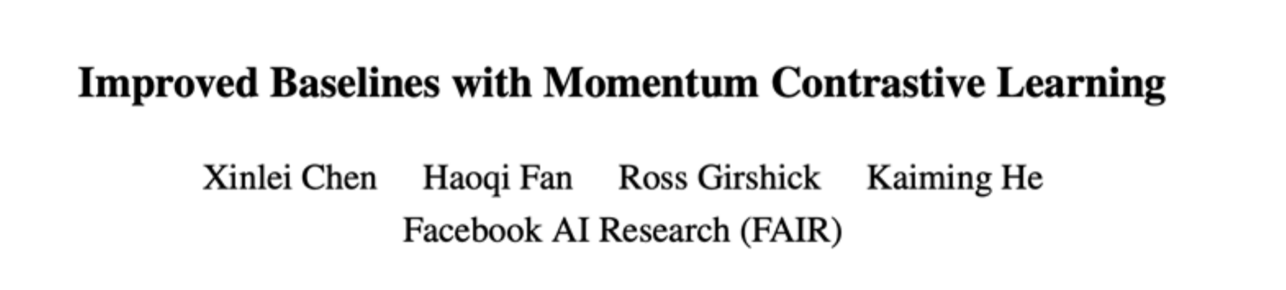
A hybrid of ideas from SimCLR and MoCo:
- From SimCLR: non-linear projection head and strong data augmentation.
- From MoCo: momentum-updated queues that allow training on a large number of negative samples (no TPU required!).
Slide from Stanford CS231n (2026), Lecture 12, p. 84. Paper: X. Chen et al. (2020).
B · Instance contrastive learning: SimCLR and MOCO
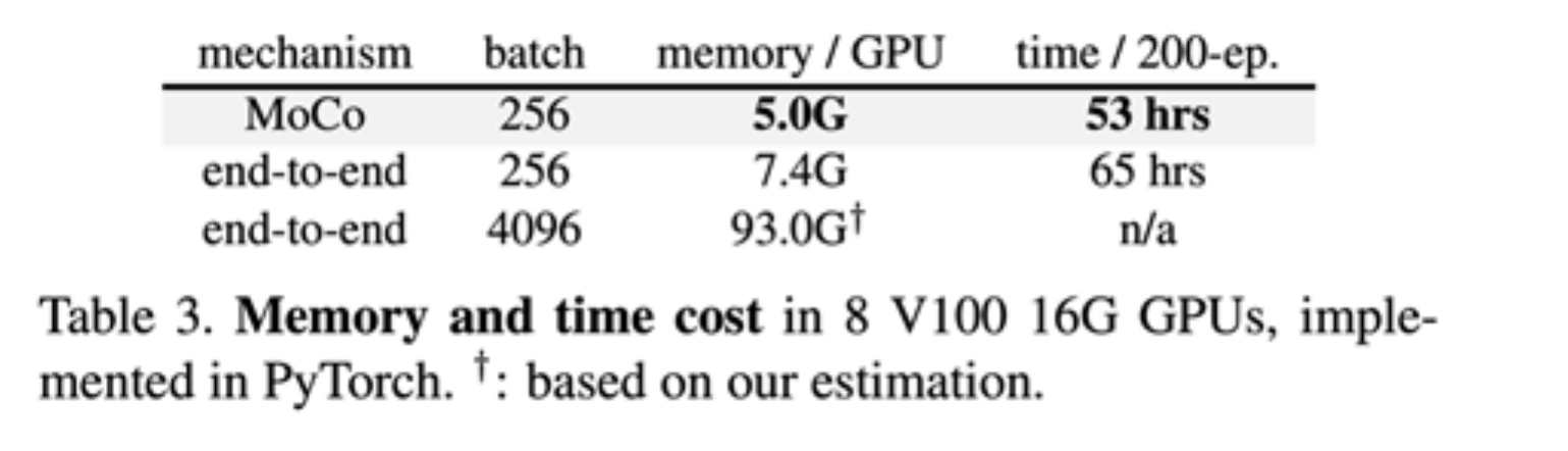
MoCo vs. SimCLR vs. MoCo V2
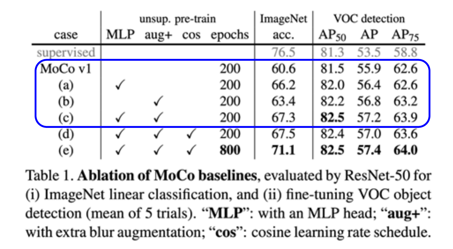
Key takeaways:
- Non-linear projection head and strong data augmentation are crucial for contrastive learning.
Slide from Stanford CS231n (2026), Lecture 12, p. 85. Table: X. Chen et al. (2020), Table 1.
B · Instance contrastive learning: SimCLR and MOCO
MoCo vs. SimCLR vs. MoCo V2
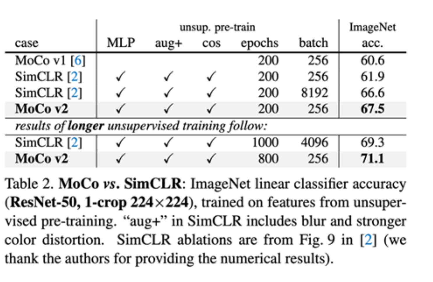
Key takeaways:
- Non-linear projection head and strong data augmentation are crucial for contrastive learning.
- Decoupling mini-batch size with negative sample size allows MoCo-V2 to outperform SimCLR with smaller batch size (256 vs. 8192).
Slide from Stanford CS231n (2026), Lecture 12, p. 86. Table: X. Chen et al. (2020), Table 2.
B · Instance contrastive learning: SimCLR and MOCO
MoCo vs. SimCLR vs. MoCo V2
Key takeaways:
- Non-linear projection head and strong data augmentation are crucial for contrastive learning.
- Decoupling mini-batch size with negative sample size allows MoCo-V2 to outperform SimCLR with smaller batch size (256 vs. 8192).
- … all with much smaller memory footprint! (“end-to-end” means SimCLR here)
Slide from Stanford CS231n (2026), Lecture 12, p. 87. Table: X. Chen et al. (2020), Table 3.
B · Sequence contrastive learning: CPC
Instance vs. Sequence Contrastive Learning
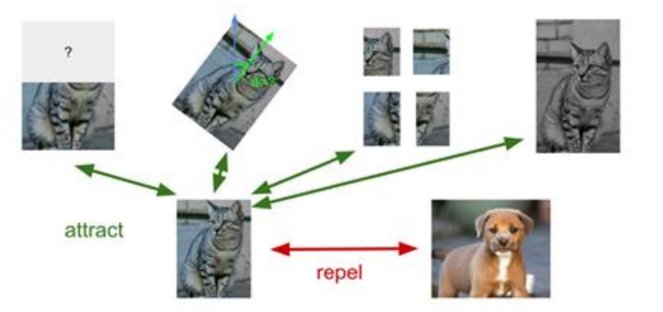
Instance-level contrastive learning:
contrastive learning based on positive & negative instances.
Examples: SimCLR, MoCo
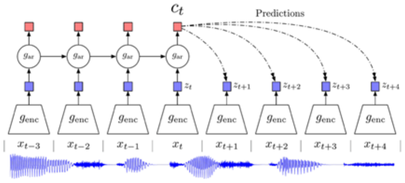
Sequence-level contrastive learning:
contrastive learning based on sequential / temporal orders.
Example: Contrastive Predictive Coding (CPC)
Slide from Stanford CS231n (2026), Lecture 12, p. 88. Right figure: van den Oord et al. (2018), Fig. 1.
B · Sequence contrastive learning: CPC
Contrastive Predictive Coding (CPC)
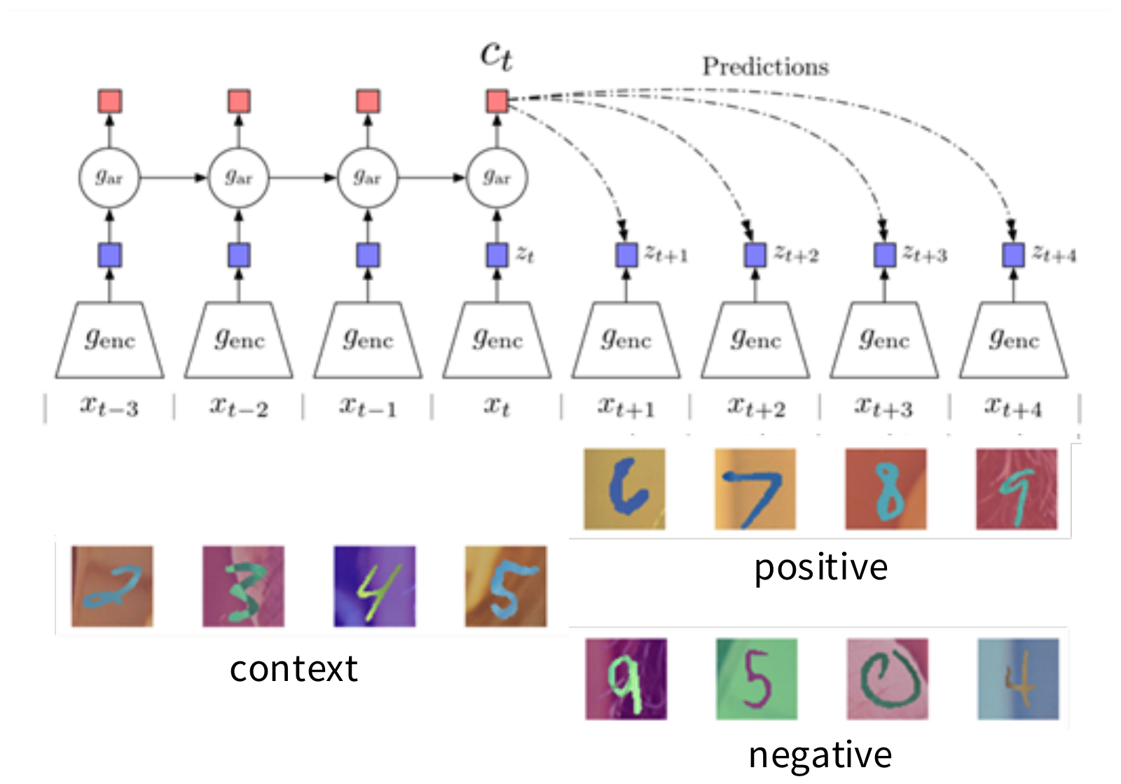
Contrastive: contrast between “right” and “wrong” sequences using contrastive learning.
Predictive: the model has to predict future patterns given the current context.
Coding: the model learns useful feature vectors, or “code”, for downstream tasks, similar to other self-supervised methods.
Slide from Stanford CS231n (2026), Lecture 12, p. 89. Figure: van den Oord et al. (2018); the deck adds a “Figure source” link.
B · Sequence contrastive learning: CPC
Contrastive Predictive Coding (CPC)
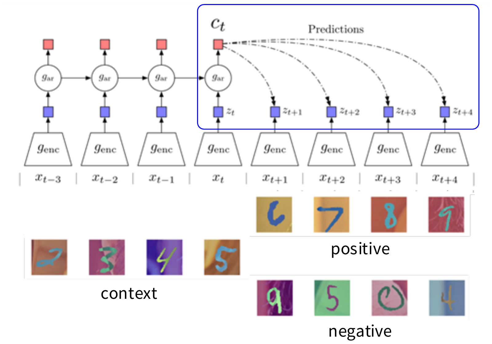
- Encode all samples in a sequence into vectors \(z_t = g_{enc}(x_t)\)
- Summarize context (e.g., half of a sequence) into a context code \(c_t\) using an auto-regressive model \((g_{ar})\). The original paper uses GRU-RNN here.
- Compute InfoNCE loss between the context \(c_t\) and future code \(z_{t+k}\) using the following time-dependent score function: \[s_k(z_{t+k}, c_t) = z_{t+k}^T W_k c_t\] where \(W_k\) is a trainable matrix.
Slide from Stanford CS231n (2026), Lecture 12, pp. 90–92. One animation; its final state (“The original paper uses GRU-RNN here.” is on p. 91 only). Math retyped. Figure: van den Oord et al. (2018).
B · Sequence contrastive learning: CPC
CPC example: modeling audio sequences
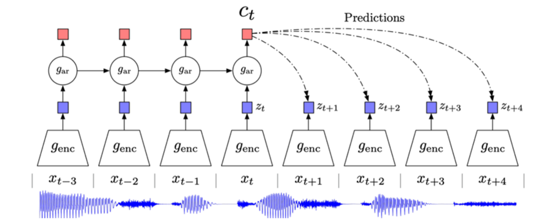
Slide from Stanford CS231n (2026), Lecture 12, p. 93. Figure: van den Oord et al. (2018), Fig. 1.
B · Sequence contrastive learning: CPC
CPC example: modeling audio sequences
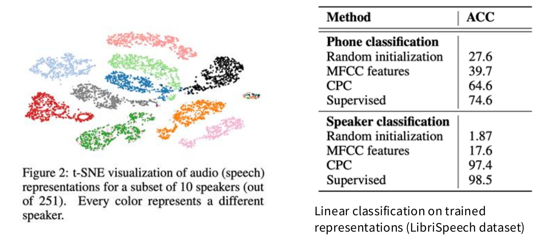
Slide from Stanford CS231n (2026), Lecture 12, p. 94. Figure and table: van den Oord et al. (2018), Fig. 2 and Table 1.
B · Sequence contrastive learning: CPC
CPC example: modeling visual context
Idea: split image into patches, model rows of patches from top to bottom as a sequence. I.e., use top rows as context to predict bottom rows.
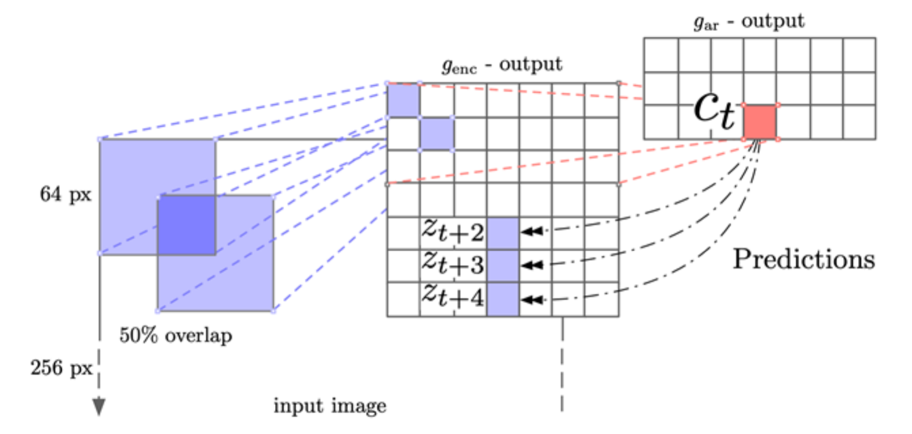
Slide from Stanford CS231n (2026), Lecture 12, p. 95. Figure: van den Oord et al. (2018), Fig. 4.
B · Self-Distillation Without Labels, DINO
DINO: Self-Distillation with No Labels
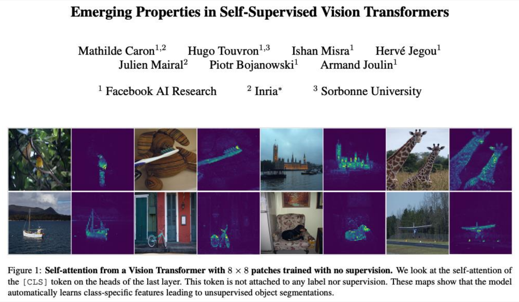
Slide from Stanford CS231n (2026), Lecture 12, p. 96. Figure: Caron et al. (2021), Fig. 1.
B · Self-Distillation Without Labels, DINO
DINO
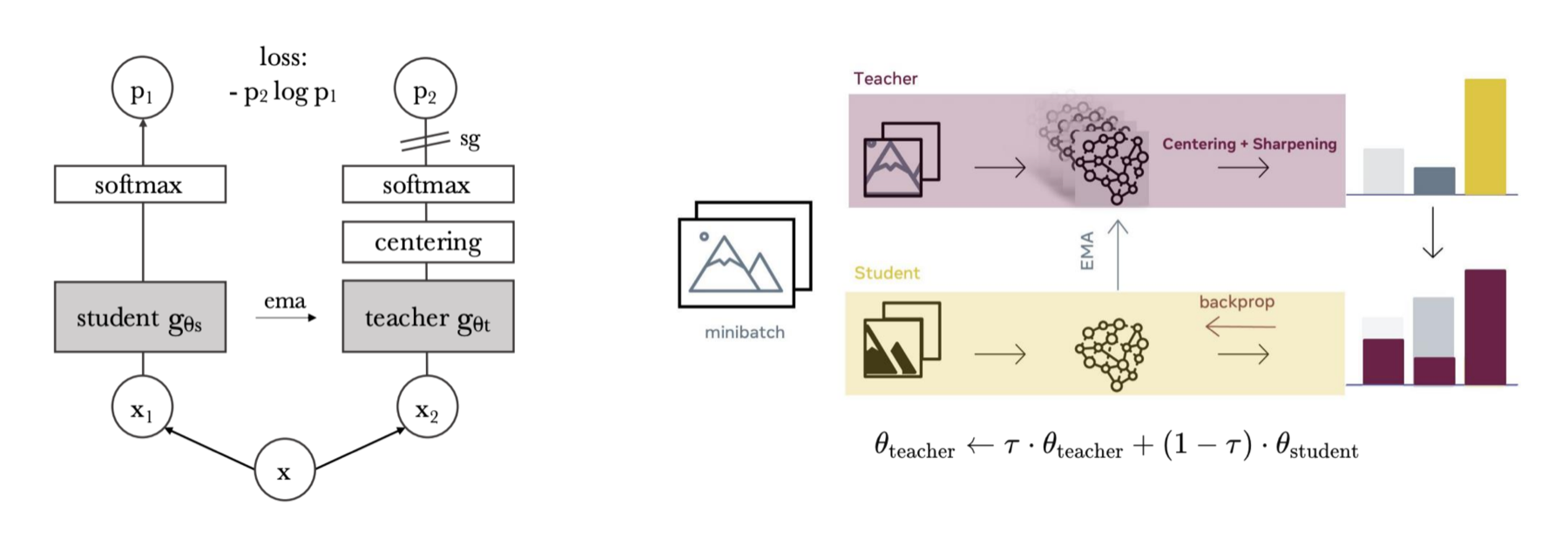
Teacher update (EMA): \(\theta_{teacher} \leftarrow \tau\,\theta_{teacher} + (1-\tau)\,\theta_{student}\). At each step the teacher weights move slowly toward the student weights. \(\tau\) is close to 1 (0.996). Only the student is trained.
Why: the teacher is an average of past students, so its targets are steadier and better than the student's own. Copying the student weights into the teacher fails to converge.
B · Self-Distillation Without Labels, DINO
DINO
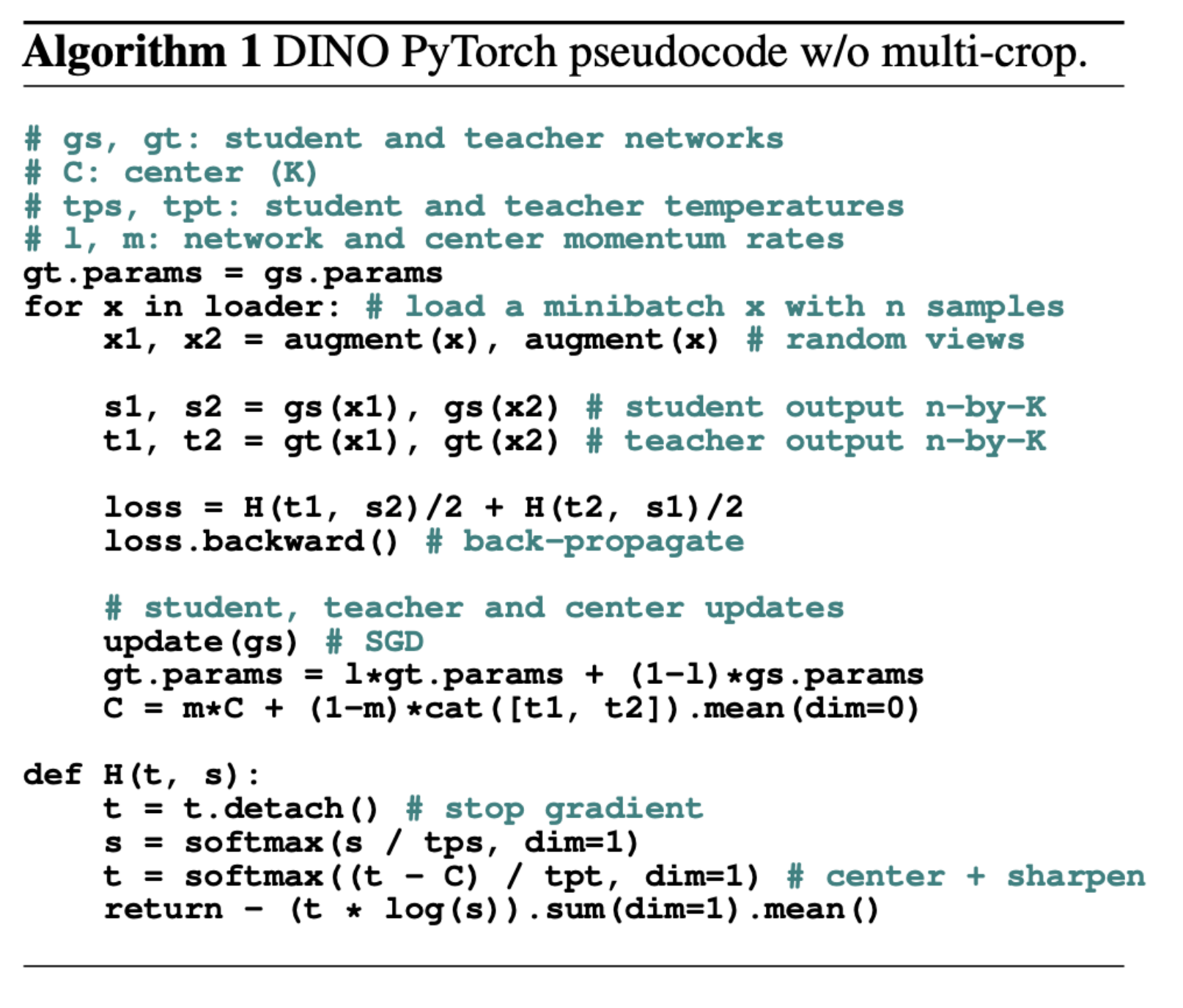
Slide from Stanford CS231n (2026), Lecture 12, p. 98. Figure: Caron et al. (2021), Algorithm 1.
B · Self-Distillation Without Labels, DINO
DINO v2
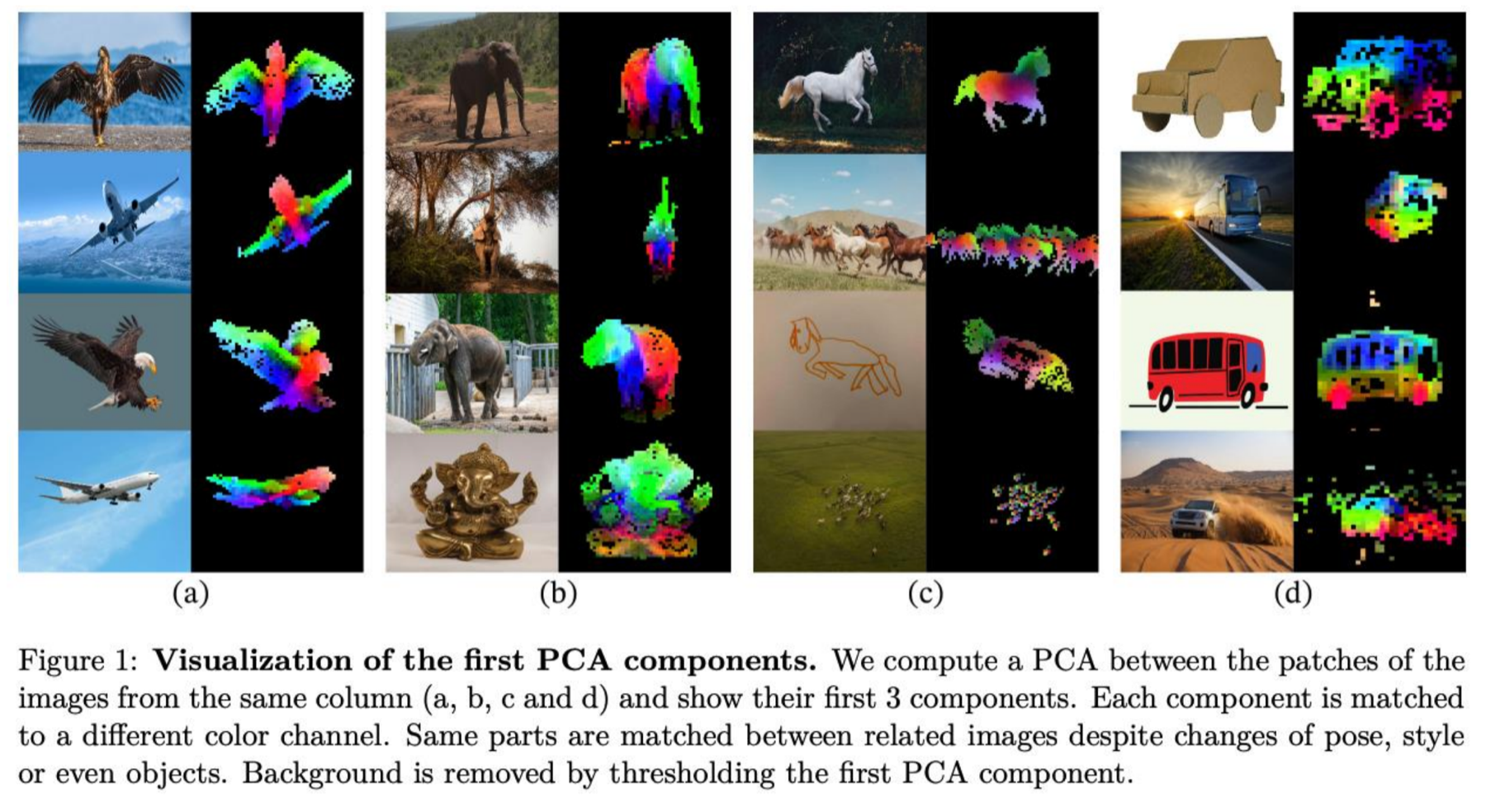
Slide from Stanford CS231n (2026), Lecture 12, p. 99. The deck credits Caron et al. (2021); the figure is Oquab et al. (2024), Fig. 1 (DINOv2).
B · Self-Distillation Without Labels, DINO
Summary: Contrastive Representation Learning
SimCLR: a simple framework for contrastive representation learning
- Key ideas: non-linear projection head to allow flexible representation learning
- Simple to implement, effective in learning visual representation
- Requires large training batch size to be effective; large memory footprint
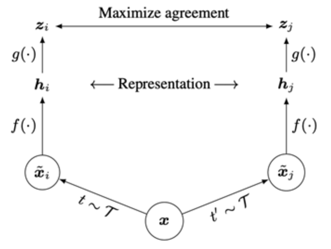
Slide from Stanford CS231n (2026), Lecture 12, p. 101. Figure: T. Chen et al. (2020), Fig. 2.
B · Self-Distillation Without Labels, DINO
Summary: Contrastive Representation Learning
MoCo (v1, v2): contrastive learning using momentum sample encoder
- Decouples negative sample size from minibatch size; allows large batch training without TPU
- MoCo-v2 combines the key ideas from SimCLR, i.e., nonlinear projection head, strong data augmentation, with momentum contrastive learning
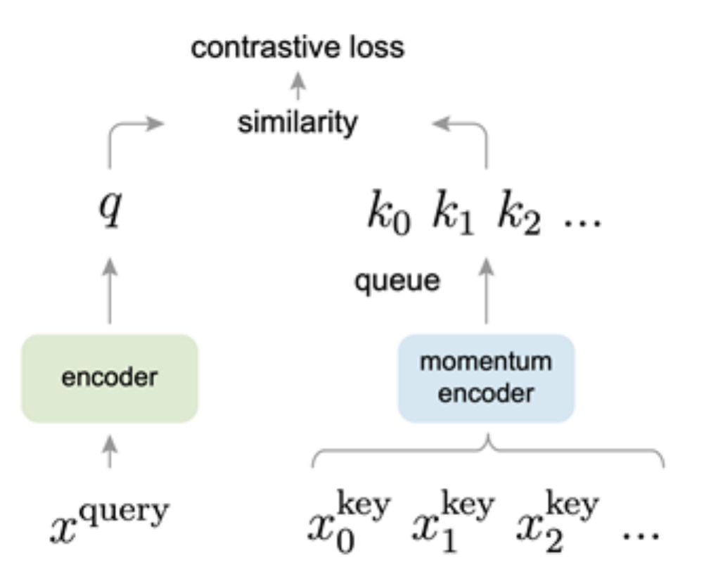
Slide from Stanford CS231n (2026), Lecture 12, p. 102. Figure: He et al. (2020), Fig. 1.
B · Self-Distillation Without Labels, DINO
Summary: Contrastive Representation Learning
CPC: sequence-level contrastive learning
- Contrast “right” sequence with “wrong” sequence.
- InfoNCE loss with a time-dependent score function.
- Can be applied to a variety of learning problems, but not as effective in learning image representations compared to instance-level methods.
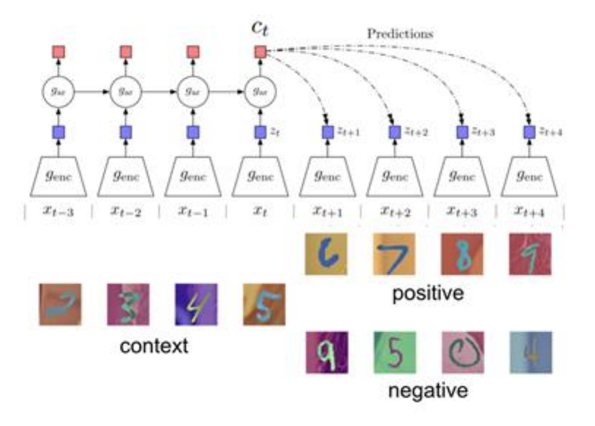
Slide from Stanford CS231n (2026), Lecture 12, p. 103. Figure: van den Oord et al. (2018).
C
The problem: dense features degrade during long training

- Each map: cosine similarity between the patch marked with a red cross and every other patch, at increasing training iterations
- Global metrics (ImageNet linear probe) keep improving the whole time
- Patch-level maps get noisier and less localized
- Global and dense performance are decoupled: the global objective progressively dominates, and the patch-level iBOT loss cannot hold the balance
- This is why “just train longer / bigger” had stopped paying off for dense tasks
Slide from Georgia Tech CS 8803-VLM (2026), Lecture 3, p. 48. Figure: Siméoni et al. (2025), Fig. 6; panels cropped from the deck page.
C
The fix: Gram anchoring
- Idea: regularize the structure of patch-to-patch similarities
- Let \(X_s\), \(X_G\) be the \(P{\times}d\) matrices of L2-normalized patch features of the student and of a Gram teacher — an earlier EMA checkpoint whose dense maps were still clean
\(L_{\text{Gram}} = \lVert X_s X_s^{\top} - X_G X_G^{\top} \rVert_F^2\)
- Because the loss only constrains the Gram matrix, individual features are free to keep moving
- Applied as a refinement stage after 1M iterations; the Gram teacher is refreshed every 10k iterations
- Remarkably, it repairs already-degraded maps rather than merely preventing the damage
- \(L_{\text{Ref}} = w_D\cdot L_{\text{DINO}} + L_{\text{iBOT}} + w_{DK}\cdot L_{\text{DKoleo}} + w_{\text{Gram}}\cdot L_{\text{Gram}}\)
- ADE20k dense linear probe: 50.3 → 55.7 mIoU; NYU depth RMSE 0.307 → 0.281, with ImageNet linear unchanged
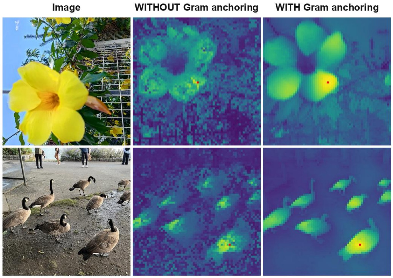
Slide from Georgia Tech CS 8803-VLM (2026), Lecture 3, p. 49. Page cites Siméoni et al. (2025), §4.2 and Fig. 10. Panels cropped; formulas retyped.